Outsourced Emissions: Why Local Governments Should Track and Measure Consumption-Based Greenhouse Gases

While many local governments track greenhouse gas (“GHG”) emissions, almost all of them exclude most GHGs associated with consumption. These consumption-based emissions stem from the lifecycle production, pre-purchase transportation, sale, and disposal of goods, food, and services produced outside of a local jurisdiction but consumed inside the jurisdiction. Based on the limited data measuring extraterritorial emissions, these consumption-based emissions amount to more than half—and in some places more than three-fourths—of GHG emissions directly connected to local consumption patterns and behaviors. This Article argues that local governments should track and measure these pervasive GHGs. Doing so may unlock meaningful information about our carbon footprint that can be leveraged to build more effective climate mitigation strategies.

This Article is most concerned with how the dramatic undercounting of GHG emissions at the local level and the proliferation of GHG emissions associated with consumption can lead to both under- and over-regulation at the local level. This Article argues that local governments should track and measure consumption-based GHGs for four reasons. First, given the voluminous amount of GHGs associated with urban consumption, there are significant opportunities to mitigate GHG emissions. In order to do so, local communities must have the correct information. Second, failing to measure these GHGs can lead to inaccurate and inefficient regulation. Third, regulating GHGs in the absence of consumption-based information may penalize local production. Finally, measuring local consumption-based GHGs may provide the necessary information leading to more politically feasible and equitable regulation. In conclusion, tracking and measuring consumption-based GHGs at the local level should be part of any meaningful GHG reduction strategy.

PDF: Rosenbloom, Outsourced Emissions.

Introduction

Consumption-based greenhouse gas (GHG) emissions are those GHGs emitted during the lifecycle of something consumed.^[1] Take, for example, a hamburger.^[2] The purchase of a hamburger in any city, town, or county is associated with GHGs emitted during the upstream lifecycle of the hamburger.^[3] These GHGs include enteric methane, nitrous oxide associated with manure, and carbon dioxide. GHGs are emitted during several lifecycle stages of beef, including weaning, grazing, feeding, transporting cattle to sale and slaughter, processing and packaging, and sale and shipping.^[4] GHGs emitted during many of the lifecycle phases typically occur outside the locality where the beef is consumed. In many local jurisdictions, these extraterritorial emissions make up most of the GHG emissions stemming from local communities;^[5] yet they are not tracked or measured, even though dozens of localities claim to track their emissions.^[6]

While researching local GHG emissions, I found that although many local governments compile GHG inventories,^[7] almost all of these inventories do not include most GHGs associated with local consumption. The GHGs local governments choose to track and measure result in a significant discrepancy between the reported per capita GHG emissions at the local level and those at the national level. As shown in the chart below, GHG emissions for three of the most populous local governments in the United States indicate that per capita emissions—shown in the darker shade below—are reported to be lower than one-third of the national average.^[8]

The large difference between the per capita emissions on the national level versus those reported in local communities piqued my curiosity. Where were the missing GHGs? Why was there such a large mismatch between the GHG levels reported in local inventories and the levels reported in their national counterparts? I found it hard to believe that citizens in New York, Los Angeles, and Chicago, representing about 7% of the U.S. population,^[9] conducted their lives in a way that resulted in two to four times fewer carbon emissions than the U.S. average. The difference, I learned, had less to do with mass efficiencies involved with living in New York, Los Angeles, or Chicago, and more to do with the way localities report their GHG emissions.

In fact, the difference between the United States and local per capita emissions can in large part be explained by the exclusion of most consumption-based emissions from local inventories measuring GHGs. The four inventories cited above (United States, Los Angeles County, New York City, and Chicago) are “Sector-based Inventories.”^[10] These inventories primarily consist of (1) emissions associated with the consumption of products within a given boundary, and (2) emissions associated with local energy use.^[11] The inventories do not measure extraterritorial emissions associated with consuming something in the boundary that was produced, processed, transported, or disposed of outside the boundary.

The U.S. inventory includes emissions for products consumed in the United States but excludes those that are emitted in foreign countries during their lifecycle. For example, the emissions involved with electronics manufactured in China and purchased in the United States are not counted in the U.S. Sector-based Inventory. However, the emissions associated with the weaning, grazing, transporting, and other lifecycle phases of a hamburger purchased in Boston, Massachusetts, originating from cattle raised in Nebraska and processed in Illinois, would be captured in in its entirety only in the U.S. Sector-based Inventory.

By contrast, the local inventories exclude extraterritorial emissions released during the lifecycle of something consumed in the locality. Thus, Boston’s inventory would not include the upstream emissions associated with the hamburger’s lifecycle (unless one of the lifecycle stages preceding consumption also occurred in Boston). The U.S. inventory captures many of the emissions that would not have been accounted for in the local Sector-based Inventories because its jurisdictional boundary is so much larger.

Further, because most communities in the United States track GHGs through a sector-based approach, they do not measure or track consumption-based GHGs, which can make up the majority of GHG emissions associated with their citizens’ choices and behaviors.^[12] The failure to measure and track consumption-based GHGs results in underestimating, and undervaluing the importance of, consumption and consumption-based emissions. Of the almost 39,000 U.S. local governments, only three track consumption and consumption-based GHG emissions, while all others, like New York City, Los Angeles County, and Chicago, do not.^[13] Further, these local Sector-based Inventories often do not acknowledge that consumption-based GHGs are omitted.^[14] Many inventories imply that the sector-based approach captures all local GHG emissions, potentially leading readers to conclude that the inventory is all-encompassing.

The three Consumption-Based Emission Inventories (“Consumption-based Inventory”) track emissions stemming from the lifecycle production, pre-purchase transportation, sale, and disposal of goods, food, and services produced outside of a local jurisdiction but consumed inside the jurisdiction.^[15] Those inventories indicate that a consumption-based GHG accounting can be three to four times higher than a sector-based GHG accounting.^[16] While there are justifications for performing and regulating pursuant to local Sector-based Inventories,^[17] this Article argues that local governments should also track and measure consumption-based GHGs. Doing so may unlock meaningful information about our carbon footprint that can be leveraged to build more effective climate mitigation strategies. This is not to say that sector-based GHG emissions should not be tracked and measured. Rather, whether a local government should track and measure consumption-based emissions, sector-based emissions, or both depends on a variety of factors. Such factors are discussed below and include whether that community is a net exporter or importer of goods or GHGs, whether it has the funds to perform the inventory, and how difficult it would be to obtain the information necessary to perform the inventory.^[18]

The issue of whether local governments should track and measure consumption-based GHGs has not yet been explored. Related scholarship has primarily addressed two important areas: (1) ethical and legal obligations concerning consumption and associated GHG emissions,^[19] and (2) policies to generally reduce GHG emissions at the local level.^[20] Scholarship in the first area does not include an exploration of the fact that the majority of localities do not track or measure local consumption-based GHGs.^[21] Scholarship in the second area typically explores reducing GHGs through buildings, waste, and water without addressing consumption patterns and behaviors at the local level or the importance of Consumption-based Inventory data.^[22] Scholarship to date has not explored the combination of these two areas of research to identify reduction strategies at the local level designed to address mass consumption and consumption-based GHG emissions.

It is critical to begin this Article with a review of local Consumption-based Inventories because such a review reveals the importance of regulating consumption-based GHGs.^[23] As such, Part I explains how Consumption-based Inventories and Sector-based Inventories are structured and what they measure. This Part takes a deep dive into the two ways local governments measure GHG emissions.

Part II then compares Consumption-based Inventories and Sector-based Inventories, with particular focus on their different results and methodologies. Among other things, the comparison shows that, in some jurisdictions, consumption-based emissions can dwarf sector-based emissions. This Part illustrates that many communities across the country are drastically undercounting their GHG emissions. Further, measuring consumption-based emissions provides critical data relevant to behaviors and inequities involved with wealth, consumption, and GHG emissions.

Part III identifies four reasons why local governments should track and measure GHGs. First, urban areas are hubs associated with GHG emissions—most of which are consumption-based—providing ample opportunity to explore mitigation strategies. Second, failing to measure consumption-based GHGs may dramatically skew the information serving as the basis for local regulation and may lead to inaccurate or ineffective policies. Third, regulating based solely on sector-based information and inventories may penalize local production. Fourth, measuring local consumption-based GHGs may lead to more politically feasible and equitable regulation.

This Article is most concerned with the proliferation of GHG emissions associated with consumption and the inequities involved with those emissions.^[24] While it concludes that local governments should track and measure consumption-based GHGs, it does not suggest that this local measure should substitute for state and federal governments doing the same. However, as long as climate change policy at all levels of government fails to effectively address the root of the problem, tracking and measuring consumption-based GHGs is one way that local communities can be informed about—and therefore act to reduce—the GHGs associated with their behaviors. Local governments are an untapped resource that are well situated to address consumption-based GHGs. At a time where the devastating effects of climate change are already being felt worldwide, we need new, innovative, and aggressive solutions to address the problems created by GHG emissions—a challenge perfectly tailored to local communities.

I. Description of Sector-Based and Consumption-Based GHG Emission Inventories

Sector-based and Consumption-based Inventories are different ways to measure and track GHG emissions associated with a specific jurisdiction. Sector-based Inventories are by far the predominant approach, with only three local governments relying on Consumption-based Inventories.^[25] Both Sector-based Inventories and Consumption-based Inventories are designed to provide a picture of GHG sources and can “serve[] as a starting point for developing and monitoring results of strategies that can effectively reduce GHG emissions.”^[26] This Part explains the two types of inventories in order to provide perspective and background on which GHGs are measured in each type of inventory.

A. Sector-Based Inventories

Dozens of local governments have performed Sector-based GHG Inventories.^[27] Sector-based Inventories typically account for certain GHGs stemming from specific sources which physically originate in the jurisdiction and GHGs associated with electricity—even if that electricity is generated outside of the jurisdiction.^[28] Structuring Sector-based Inventories requires local governments to (1) set the boundary (e.g., the municipal boundaries) and the relevant time frame (e.g., calendar year 2020) in which GHGs will be measured, (2) to determine which GHGs will be measured (e.g., CO₂), and (3) to select the sources to be accounted in the boundary (e.g., residential buildings).

1. Establishing Inventory Boundary and Time Frame

In recent years, local governments have tried to make Sector-based Inventories consistent with each other. One methodology that drives numerous local Sector-based Inventories is the Global Protocol for Community-Scale Greenhouse Gas Emissions Inventories (“GPC”).^[29] The GPC suggests that local governments begin by defining an inventory boundary and relevant time in which GHGs will be measured.^[30] For example, both Chicago’s 2015 and Washington D.C.’s 2012–13 Sector-based Inventories set the city limits as the designated relevant area and a one-year time frame for measuring emissions.^[31]

2. Determining Emissions to be Tracked

In addition to selecting boundaries, local governments must also select which GHGs will be measured in their Sector-based Inventories.^[32] Chicago’s 2015 inventory, for example, measured “carbon dioxide (CO₂), methane (CH₄), nitrous oxide (N₂O), hydrofluorocarbons (HFCs), perfluorocarbons (PFCs), sulphur hexafluoride (SF₆) and nitrogen trifluoride (NF₃)”^[33] while Washington D.C.’s inventory measured CO₂, CH₄, and N₂O.^[34] Most inventories convert GHGs to equivalent CO₂ (CO₂e).

3. Selecting Sources to be Accounted in the Boundary

For sources or sectors, the GPC identifies the following sectors (in capital letters) and subsectors from which GHGs could or should be measured:

Table 1

Sectors and subsectors

STATIONARY ENERGY

Residential buildings

Commercial and institutional buildings and facilities

Manufacturing industries and construction

Energy industries

Agriculture, forestry, and fishing activities

Non-specified sources

Fugitive emissions from mining, processing, storage, and transportation of coal

Fugitive emissions from oil and natural gas systems

TRANSPORTATION

On-road

Railways

Waterborne navigation

Aviation

Off-road

WASTE

Solid waste disposal

Biological treatment of waste

Incineration and open burning

Wastewater treatment and discharge

INDUSTRIAL PROCESSES AND PRODUCT USE

Industrial processes

Product use

AGRICULTURE, FORESTRY AND OTHER LAND USE

Livestock

Land

Aggregate sources and non-CO2 emission sources on land

Not all inventories measure all sectors set forth in the GPC. Chicago’s inventory, for example, excludes both energy relating to agricultural activities and GHG’s stemming from agricultural activities. Chicago’s list of sources includes:

Table 2^[35]

Sectors and subsectors

STATIONARY ENERGY

Residential buildings

Commercial and institutional buildings and facilities

Manufacturing industries and construction

Fugitive emissions from oil and natural gas systems

TRANSPORTATION

On-road

Railways

Waterborne navigation

Aviation

Off-road

WASTE

Solid waste disposal

Biological treatment of waste

Incineration and open burning

Wastewater treatment and discharge

A typical Sector-based Inventory has three “scopes” of GHG emissions:

Scope 1 emissions come directly from sources in the local jurisdiction (typically including fossil fuel combustion).^[36]

Scope 2 emissions result indirectly from purchased electricity. Scope 2 emissions are “indirect” because they occur outside the locality and “physically occur at the facility where electricity is generated.”^[37]

Scope 3 emissions are indirect emissions other than Scope 2 emissions (these are typically the upstream lifecycle emissions included in a Consumption-based Inventory, such as waste disposal).^[38] Scope 3 emissions are an optional reporting category, stemming from sources and activities outside a locality’s boundary but are a consequence of local activities.^[39] Many local inventories do not include Scope 3 emissions or only include a small subset of them.^[40]

Even before local governments made efforts to systemize the methodologies across Sector-based Inventories, most Sector-based Inventory results looked surprisingly similar. A typical Sector-based Inventory lists “stationary energy” as the large majority of GHGs, with “residential buildings” and “commercial and institutional buildings and facilities” being the largest sector-based emissions.^[41] In Sector-based Inventories, transportation typically amounts to the second-highest amount of GHG emissions, with waste ranked third, accounting for only a small percentage of sector-based GHG emissions.^[42] For example, Washington, D.C.’s inventory found buildings amounted to 75% of emissions, which were followed by transportation (21%) and emissions stemming from landfills and other forms of decomposing waste (4%).^[43]

Similarly, Chicago’s 2015 inventory concluded that stationary energy emissions accounted for 72%^[44] of total emissions; transportation emissions contributed 25%, and waste emissions 3%.^[45] This 2015 inventory indicated that the highest emitting subsectors were:

residential buildings (28%),

commercial and institutional buildings and facilities (25.7%),

manufacturing industries and construction (17.1%), and

on-road transportation (15.6%).^[46]

This Subpart ends with a typical sector-based summary table (Table 3), setting forth all subsections in Chicago’s Sector-based Inventory. Of particular note for these purposes is that Scope 1 emissions amounted to 51.5% of GHG emissions; Scope 2 emissions amounted to 45%; and Scope 3 emissions, the extraterritorial emissions, amounted to less than 4% of the total 2015 GHG emissions.^[47] It also highlights the importance of residential and commercial buildings, which amount to over one-half of the sector-based emissions measured. The limited scope of the sector-based analysis compels the reader to believe that residential and commercial buildings are the largest sources of GHGs. But, as discussed below in Part III, Consumption-based Inventories indicate that residential and commercial buildings emit significantly fewer GHGs than numerous consumption-based sources.^[48]

Table 3

 

Sector		Emissions MT CO2e‌/year for Chicago			% of Total
	Scope 1	Scope 2	Scope 3	BASIC Total
Stationary Energy	9,018,535	14,481,547	0	23,500,082	72.0%
Residential Buildings	5,264,148	3,863,687		9,127,835	28.0%
Commercial and Institutional Buildings and Facilities	2,699,359	5,679,497		8,378,856	25.7%
Manufacturing Industries and Construction	781,710	4,811,717		5,593,427	17.1%
Energy Industries	28	NA		28	0.0%
Water Conveyance and Treatment	46,774	51,554		98,327	0.3%
Calumet WWTP Wastewater Conveyance	2,390	75,093		77,482	0.2%
Fugitive Emissions from Oil and Natural Gas Systems	224,126	NA		224,126	0.7%
Transportation	7,763,715	284,748	0	8,048,463	24.6%
On-road Transportation	5,100,066	NA		5,100,066	15.6%
Railways	109,459	284,748		394,207	1.2%
Waterborne Navigation	4,366	NA		4,366	0.0%
Aviation	1,551,941	NA		1,551,941	4.8%
Off-road Transportation	997,883	NA		997,883	3.1%
Waste	2,235	0	1,100,599	1,102,834	3.4%
Solid Waste Generated in the City	NO		998,888	998,888	3.1%
Biological Waste Generated in City	NO		112	112	0.0%
Wastewater Treatment and Discharge	2,235		101,599	103,835	0.3%
TOTAL	16,784,486	14,766,295	1,100,599	32,651,379	100.0%

B. Consumption-Based Inventories

In addition to compiling Sector-based Inventories, three local governments—Multnomah County, Oregon; San Francisco, California; and King County, Washington—also completed Consumption-based Inventories.^[49] A Consumption-based Inventory “attributes carbon emissions based primarily on the local consumption of goods and services, regardless of where those goods were produced.”^[50] The common definition of a Consumption-based Inventory is one that includes all emissions associated with the lifecycle of things consumed.^[51] Based on national economic theory, the “consumers” associated with Consumption-based Inventories include households, governments, and businesses when investing in capital, such as in equipment (for example, a tractor or refrigerator).^[52]

Like Sector-based Inventories, Consumption-based Inventories can vary in methodology.^[53] Structuring a Consumption-based Inventory requires local governments to set the boundary in which consumption will be measured, determine which consumed products will be measured, select the lifecycle phases of those products that will be included in the accounting, identify which GHGs will be measured during those phases, and create a time frame from which to measure GHGs.

Understanding emissions covered in Consumption-based Inventories is helped by a comparison to “embedded emissions.” Emissions measured in Consumption-based Inventories are similar to embedded emissions, but are simultaneously a bit broader and narrower than embedded emissions.^[54] Typically, embedded emissions include all upstream emissions associated with manufacturing a product.^[55] The emissions covered in a Consumption-based Inventory, by contrast, are broader in that they also cover “use,” where embedded emissions do not. For example, both emissions in a Consumption-based Inventory and embedded emissions include emissions associated with the manufacturing and transporting of a car. However, while emissions in a Consumption-based Inventory include the use of that car, embedded emissions do not. A Consumption-based Inventory and an Embedded-emissions Inventory for King County, Washington, would include the emissions associated with the manufacturing of a car purchased by a citizen of King County. The Consumption-based Inventory, however, would also include emissions associated with the use of that car by that citizen.^[56]

Consumption-based Inventory coverage can also be narrower than embedded emissions. This difference is particularly relevant when measuring emissions stemming from non-consumers, such as restaurants, where the food is consumed by the patron and not the restaurant itself. As mentioned above, Consumption-based Inventories generally do not include emissions associated with businesses when not investing in capital;^[57] however, an embedded emission inventory would include these emissions. For example, if a King County restaurant purchased hamburgers, the upstream emissions associated with the hamburgers would not be included in the King County Consumption-based Inventory—unless a King County resident frequenting that restaurant purchased the hamburger. In contrast, the emissions would be included in an “Embedded-emission Inventory.” Yet, to date, no local government has conducted such an inventory.

The following three Subparts describe three ways to understand Consumption-based Inventory emissions. Consumption-based Inventory emissions can help identify (1) consumed products that result in high emissions (e.g., food and beverages or appliances), (2) life cycle phases of high emissions (e.g., production or use), and (3) consumers of high emissions (e.g., household or government).

1. Consumption-Based Inventory Emissions By Product Consumed

The three localities that compile Consumption-based Inventories track GHGs stemming from dozens of goods (e.g., clothes and electronic equipment), food, and services consumed by citizens within the jurisdiction.^[58] Whereas Sector-based Inventories track GHGs by source, such as residential, commercial, or industrial buildings, Consumption-based Inventories track GHGs by the type of product consumed or used, such as concrete, electronics, and healthcare.^[59]

The three Consumption-based Inventories measured GHGs from the consumer’s point of view focusing on products^[60] (1) produced in the jurisdiction and sold in the jurisdiction^[61] and (2) produced outside the jurisdiction and sold inside the jurisdiction.^[62] San Francisco, for example, tracked data from 440 products (classified in the report as “sectors”) and categorized those products into 16 categories and 62 subcategories.^[63] Analyzing these 440 products allowed the community to delve into consumption patterns surrounding many goods.^[64] San Francisco tracked lighting fixtures, knit apparel, lime and gypsum products, among a number of other goods.^[65] Table 4 below provides the 16 categories in the left-hand column, an example of the 62 subcategories in the middle column, and an example of the 440 products in the right-hand column.^[66]

Table 4

Category	Sample Subcategory	Sample Product
Appliances, HVAC[67]	Heating and cooling appliances	Air conditioning, refrigeration, and warm air heating equip.
Appliances, other	Ranges and microwaves	Household cooking appliances
Clothing	Clothing	Men’s and boy’s cut and sewn apparel
Concrete, cement, and lime	Concrete, cement, and lime	Cement
Construction	Residential construction and remodeling	Newly constructed residential permanent site single and multifamily structures
Electronics	Computer service and equipment	Computer storage devices
Food and beverages	Poultry and eggs	Processed poultry meat products
Forest products	Paper and cardboard	Paper from pulp
Fuel, utilities, waste	Oil and gas extraction	Petrochemicals
Healthcare	Healthcare services	Offices of physicians, dentists, and other health practitioners
Home, yard, office	Home furnishings	Carpets and rugs
Retailer and wholesale	Retailers	Motor vehicle and parts
Services	Banks, financial, legal, real estate, and insurance	Real estate buying and selling, leasing, managing, and related services
Transportation services	Transportation services, air	Air transportation services
Vehicles and vehicle parts	Cars and light trucks	Automobiles
Other	Other	Plastic bottles

Consumption-based Inventories illuminate several important high GHG-emitting sources not found in the Sector-based Inventories. As seen in Table 5, the five highest emitting sources (which varied among the inventories) were food and beverages production, vehicle and parts use, appliance use, services, and other manufactured goods production.

Table 5^[68]

San Francisco, CA[69]		King County, WA[70]		Multnomah County, OR[71]
Other	4,360,000 MTCO2e	Vehicles and Vehicle Parts	12,299,000 MTCO2e	Vehicles and parts	2,822,000 MTCO2e
Food and beverage	4,250,000 MTCO2e	Food and Beverage	7,474,000 MTCO2e	Food and beverage	2,312,000 MTCO2e
Vehicles	3,270,000 MTCO2e	Services	6,214,000 MTCO2e	Appliances	2,064,000 MTCO2e
Appliances	2,050,000 MTCO2e	Appliances HVAC	5,059,000 MTCO2e	Services	1,488,000 MTCO2e
Transportation Services	1,860,000 MTCO2e	Other[72]	4,405,000 MTCO2e	Other manufactured goods	1,216,000 MTCO2e
Total Consumption-Based GHGs	21,730,000 MTCO2e	Total	58,165,000 MTCO2e	Total	15,806,000 MTCO2e

Table 5 indicates the high level of GHG emissions related to food and beverage both in the home and at restaurants. In Multnomah County’s inventory, food and beverages were responsible for 2.3 million metric tons of carbon dioxide equivalent (“MMTCO₂e”), making it the second highest emission source and amounting to approximately 15% of all consumption-based carbon emissions.^[73] Similarly, in King County the consumption of food and beverages resulted in 7.474 MMTCO₂e, making it the second highest emission source.^[74] In San Francisco’s Consumption-based Inventory, food and beverage consumption accounted for 4.25 MMTCO₂e, also making it the second-highest emission source, behind “other.”^[75]

Table 6 also illustrates that San Francisco, like King County, is responsible for more emissions stemming from “restaurants” and “red meat” than any other subcategory.^[76] Other GHG intensive subcategories in food and beverages include dairy and beverages. As shown in Table 6, almost all the 4.25 MMTCO₂e food-based emissions in San Francisco were from households, which amounted to 97% of food and beverages emissions.^[77]

Table 6

Category	GHG Emissions by Type of Consumer
	Household	Gov’t	Total
Food & Beverages	4.128	0.124	4.253
Beverages	0.484	0.002	0.486
Condiments, oils, sweeteners	0.085	0.002	0.087
Dairy	0.457	0.025	0.482
Fresh fruit, nuts, vegetables	0.214	0.002	0.215
Frozen food	0.115	0.001	0.116
Grains, baked good, cereals, roasted nuts, nut butters	0.444	0.008	0.452
Poultry and eggs	0.255	0.002	0.257
Processed fruit, nuts, vegetables	0.129	0.007	0.135
Red meat	0.700	0.038	0.738
Restaurants	0.849	0.029	0.878
Seafood	0.036	0.002	0.038
Other food and agriculture	0.361	0.006	0.368

Additionally, the purchase and use of vehicles and parts to repair vehicles was an important factor in each of the Consumption-based Inventories, ranking first or third in all Consumption-based Inventories.^[78] This category included the subcategories of aircraft, cars and light trucks, heavy duty trucks, other road vehicles, railroad rolling stock, ships and boats, and vehicle parts.^[79] Similarly, Multnomah County defined vehicles and parts to include emissions produced during the making of the vehicle or parts (regardless of where that vehicle or part was made), the use of the vehicles, pre-purchase transportation, the wholesale and retail, and postconsumer disposal.^[80]

2. Emissions By Lifecycle Phase

In addition to selecting the products to be measured, the local governments also selected the lifecycle phases that will be measured for the products. This Subpart explores the five lifecycle phases selected by the three inventories. Although worded slightly different in each inventory, the five phases are: production, prepurchase transportation, wholesale‌/retail, use, and postconsumer disposal.^[81]

Production (natural resource extraction, processing, and manufacturing) amounted to 63%, 61%, and 56% of consumption-based emissions from San Francisco, King County, and Multnomah County, respectively.^[82] Of the production-based emissions, the production of food and beverages resulted in the largest amount of GHG emissions by far. In San Francisco’s inventory, the production of food and beverages was the largest single product in any phase, amounting to almost 27% of all GHGs emitted through production and almost 17% of emissions overall.^[83] Similarly, in King County’s inventory, the production of food and beverages was the single largest product in any phase, amounting to 19% of all production-based emissions and 11.7% of emissions overall.^[84] In Multnomah County’s inventory, the production of food and beverages was surpassed only by the use of vehicles and parts.^[85] Indeed, “[m]ore than half of [Multnomah’s] consumption-based carbon emissions are generated during the production phase of the lifecycle. The transportation and sale . . . adds [sic] an additional 12 percent. On average, 68 percent of a product’s lifecycle emissions are generated before a consumer begins to use [the product].”^[86] Other significant products responsible for production-based GHGs include services, vehicles and vehicle parts, health care, construction, clothing, and electronics.^[87]

The lifecycle phase of use also resulted in a significant amount of GHG emissions. Use amounted to 20%, 28%, and 31% of emissions in San Francisco, King County, and Multnomah County, respectively.^[88] GHGs emitted during the use phase of the lifecycle came predominantly from vehicles and vehicle parts, HVAC appliances, and other appliances.^[89] That being said, many products measured in Consumption-based Inventories did not result in use-based GHG emissions. For example, in King County’s inventory, clothing, food and beverages, and concrete, cement, and lime, resulted in zero emissions during the use phase.^[90] However, vehicles and vehicle parts accounted for almost half of use-based GHG emissions and almost 10.5%, 12%, and 18% of the total GHG emissions in San Francisco, King County, and Multnomah County, respectively.^[91] As San Francisco notes:

Vehicles and vehicle parts production emissions are the emissions embedded in cars purchased in San Francisco in 2008, while this category’s use emissions are the end-use emissions from San Francisco driving in 2008. Production emissions relate only to the cars purchased in 2008; use emissions relate to all cars driven in 2008.^[92]

Multnomah County also notes the importance of use-based emissions:

Therefore, it’s valuable to understand the nature of this lifecycle phase (“use phase”). Vehicles, appliances, lighting and electronics all require energy in their use and thus are responsible for the generation of associated carbon emissions. For example, to reduce emissions from the use of a vehicle, walking and biking are the best options, followed by taking public transit and using high blends of biofuels.^[93]

Prepurchase transportation (services to transport people, transportation of final product, and others) amounted to 13%, 10%, and 10% of emissions in San Francisco, King County, and Multnomah County, respectively.^[94] In King County’s inventory, transportation services amounted to over half of prepurchase transportation, and in Multnomah it amounted to almost two-thirds.^[95] Food and beverages were the next highest, but only about one-sixth of transportation services.^[96]

Finally, for the lifecycle phase of waste, in all Consumption-based Inventories, the single largest category of postconsumer disposal (which ranged from 0.2%–2% overall) was food and beverages again.^[97] Food and beverages accounted for about half of all postconsumer disposal.^[98]

3. Emissions By Consumer

Based on the type of consumer, households are by far the largest emitters. San Francisco’s and King County’s inventory noted that households are responsible for 82% and 71% of total GHG emissions, respectively.^[99] Food and beverages were the largest category in households, amounting to 23.2% of household GHG emissions in San Francisco.^[100] In King County, households were responsible for 95% of food and beverage emissions and 80% of appliances emissions.^[101] The next highest categories were vehicles and vehicle parts (16.3%), services (10%), transportation services (9.5%), and health care (8%).^[102] From a consumer’s perspective, government was responsible for 11% of emissions and business investment was responsible for 7% of Consumption-based Inventory emissions.^[103] Of note, construction amounted to 53% of business investment emissions and electronics amounted to 29.6%.^[104]

II. Comparison of Sector-Based and Consumption-Based GHG Inventories

Part I described the methodology and details of Sector-based Inventories and Consumption-based Inventories. This Part compares the two inventories to demonstrate that they produce vastly different pictures of local GHG emissions. Sector-based Inventories illustrate the production side of the economy, but not the demand side, which is the primary perspective of Consumption-based Inventories.^[105] Combined, the two help provide a more complete picture of GHGs emitted at the local level. For regions that import more embedded emissions than they export (such as most urban areas and many higher-income areas), Consumption-based Inventories provide more and better information pertaining to how we can reduce GHG emissions. For regions that export more embedded emissions (such as areas with a lot of industrial production or petroleum extraction), Sector-based Inventories provide critical information about GHG emissions. This Part further details some of the differences between the two.

A. Consumption-Based Inventories Measure Significantly More GHG Emissions

There is a significant difference between the total emissions captured in the three Consumption-based Inventories and the emissions captured in their Sector-based counterparts. Unlike a Sector-based Inventory, the Consumption-based Inventory “seeks to attribute emissions to the local consumption of goods and services (regardless of where those goods are produced.)”^[106] Consequently, consumption-based GHG accounting led to the capture and cataloging of 140%–55% more emissions than Sector-based Inventories. Relatedly, Consumption-based Inventories captured approximately 90% of total inventoried GHG emissions, compared to approximately 40% captured by Sector-based Inventories. This difference highlights the dramatic undercounting of GHG emissions occurring at the local level across the country. For example,

In Multnomah County, the Sector-based Inventory accounted for 46% of GHG emissions, while the Consumption-based Inventory accounted for 91%, an increase in measured emissions of almost 98%.^[107]

In King County, the Consumption-based Inventory revealed that “the emissions ‘footprint’ of King County’s consumption (an estimated 55 . . . [M]MTCO₂e) is significantly greater than the emissions released within King County using the [Sector-based Inventory] . . . (23 . . . [M]MTCO2e).”^[108] This difference amounts to an increase of almost 140%.

In San Francisco, the “Traditional GHG Inventory,” San Francisco’s Sector-based Inventory, resulted in 8.5 MMTCO₂e, while the Consumption-based Inventory resulted in 21.7 MMTCO₂e, amounting to an increase greater than 155% increase.^[109]

Image 1^[110] below illustrates the difference between Multnomah County’s Consumption-based Inventory and its Sector-based Inventory. Multnomah’s total GHG emissions measured were 17.3 MMTCO₂e (the sum of 9.4, 6.4, and 1.5 indicated in the Image). The Sector-based Inventory covered about 46% of the total emissions—just under half of the total measured GHGs associated with Multnomah’s citizens (7.9 MMTCO₂e equals 6.4 and 1.5 in the Image below). The Consumption-based Inventory, at 15.8 MMTCO₂e (the sum of 9.4 and 6.4 in the Image below), covered 91% of the total recorded emissions, almost twice as many as the Sector-based Inventory.^[111]

Image 1

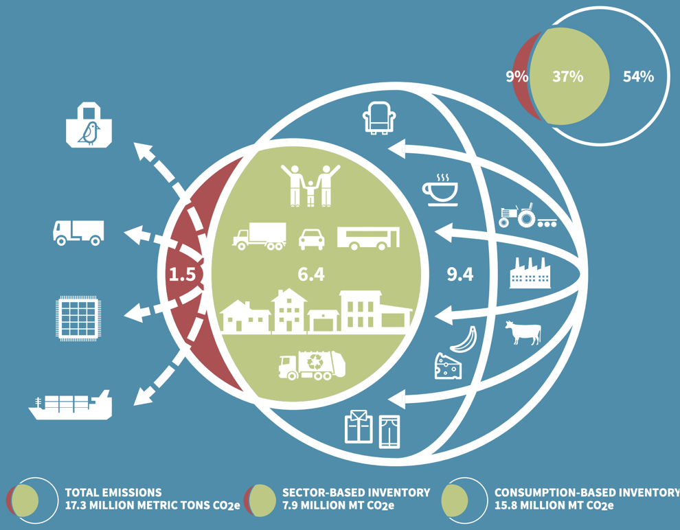
Multnomah’s Sector-based Inventory included 1.5 MMTCO₂e not covered by the Consumption-based Inventory, while the Consumption-based Inventory included 9.4 MMTCO₂e not covered by the Sector-based Inventory. The 1.5 MMTCO₂e that were not part of the Consumption-based Inventory were predominantly emissions associated with the production of a product in Multnomah County and consumed elsewhere (indicated by the dashed arrows in the small circle in Image 1, which represent goods and services flowing out of Multnomah County). The 9.4 MMTCO₂e not covered by the Sector-based Inventory are GHGs emitted outside of Multnomah County and emitted in conjunction with the lifecycle of a product consumed inside Multnomah County (indicated by the solid arrows in the large circle above, which represent goods and services flowing into Multnomah County).^[112]

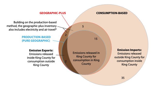
Similarly, and as illustrated in Image 2 below,^[113] King County’s Sector-based Inventory (indicated by “production-based” and “geographic plus”) included 17–24 MMTCO₂e, which amounts to 2%–41% of the total GHGs measured. In Image 2, the Sector-based Inventory included 2–4 MMTCO₂e not covered by the Consumption-based Inventory, while the Consumption-based Inventory included 35–40 MMTCO₂e not covered by the Sector-based Inventory.^[114] Like Multnomah County, the majority of consumption-based GHGs were emitted outside the local jurisdiction. In King County, this amounted to 35 MMTCO₂e associated with King County consumption.

Image 2

San Francisco’s Consumption-based Inventory (Image 3A below)^[115] included 21.7 MMTCO₂e, while its Sector-based Inventory covered 8.5 MMTCO₂e (Image 3B below).^[116] The Consumption-based Inventory tracked over two times the number of GHGs associated with San Franciscans as did the Sector-based Inventory. (For Images 3A and 3B, please see the attached PDF version of this article.)

Image 3A: Total Consumption Inventory for San Francisco (21.7 MMTCO₂)^[117]

Image 3B: Total Traditional GHG Inventory for San Francisco (8.5 MMTCO₂)^[118]

The total GHG emissions and the corresponding per capita emissions in Consumption-based Inventories are not only higher than those recorded in Sector-based Inventories but also are more reflective of U.S. emissions per capita. The chart in Section I.A. above lists the per capita emissions in the United States at 22.2 MTCO₂e. King County’s consumption-based emissions resulted in about 29 MTCO₂e per capita.^[119] “This total is more than twice as high as the [Sector-based] Inventory and about four times higher than the global average.”^[120] However, this total closely approximates the national average:

While per-person King County emissions in the [Sector-based] Inventory are much lower than for the U.S. as a whole . . . , it is striking that per-person emissions are roughly equal to the U.S. average in the Consumption-based Inventory. Per-person emissions from personal vehicle travel and residential energy (emission sources that are in both Consumption-based and Geographic-plus Inventories) are much lower in King County, but emissions associated with food, other goods, and services are higher than the U.S. average.^[121]

The bulk of the additional emissions captured by Consumption-based Inventories can be attributed to emissions stemming from goods and services produced elsewhere but consumed by local citizens.

B. Consumption-Based Inventories Provide Invaluable Details Concerning GHGs Emitted During Product Lifecycles

Digging into these overall numbers highlights important differences between Consumption-based Inventories and Sector-based Inventories. Specifically, the inventories differ in their overall approach to measuring GHGs, sources and products measured, behaviors associated with GHG emissions, and impacts on equity. Consumption-based Inventories approach measuring GHGs from a lifecycle perspective.^[122] For purposes of emissions, Consumption-based Inventories are not restricted by geography. Rather, GHGs associated with the consumption of goods are counted regardless of where they are emitted so long as they can be attributed to the lifecycle of something consumed.^[123]

[A] “consumption-based” carbon emissions inventory models carbon emissions from the full lifecycle of goods and services, including production, pre-purchase transportation, wholesale and retail, use and disposal. Whereas the Sector-based Inventory includes emissions associated with the production of goods in Multnomah County (regardless of who buys them), the [C]onsumption-based [I]nventory seeks to attribute emissions to the local consumption of goods and services (regardless of where those goods are produced).^[124]

Assume a widget manufactured in Cincinnati, Ohio, is transported to Chattanooga, Tennessee, to be utilized in the assembling of a car that is then sold in New York City, New York. Upstream emissions associated with the widget and car would not be counted in New York City’s Sector-based Inventory, even though the demand for the car came from a New Yorker. Chattanooga’s Sector-based Inventory would presumably include GHGs emitted in the manufacturing of the car but not the GHGs emitted in making the widget in Cincinnati.^[125] In this scenario, like millions of others, one person’s consumption of a good, food, or service (here, a New Yorker purchasing a car) results in GHG emissions outside the consumer’s local jurisdiction (New York City), but those emissions elude that local jurisdiction’s inventory. When viewed together, jurisdictions across the country are responsible for millions of metric tons of carbon dioxide equivalent (MTCO₂e) emissions; yet, their Sector-based Inventories reflect only a small percentage of these GHG emissions.

In terms of lifecycle phase, Sector-based Inventories are primarily—and in some cases exclusively—focused on production and, to some extent, disposal. By contrast, Consumption-based Inventories measure GHGs emitted during all phases of a product’s lifecycle. “[E]very ton of CO2‑e results from both the supply and demand side of the economic systems: it ‘belongs’ to its location of production, and it ‘belongs’ to its location of consumption.”^[126]

As noted in Part 1.B, production of consumed products amounted to 63%, 61%, and 56% of consumption-based emissions from San Francisco, King County, and Multnomah County, respectively.^[127] Only about one-third of production-based emissions occur within the local government borders.^[128] Compared to overall consumption, very little food, for example, is produced in the jurisdictions of San Francisco, King County, and Multnomah County. Yet, GHGs stemming from the production of food and beverages amounted to 11.7%–17% of all Consumption-based Inventory emissions.^[129]

In the Consumption-based Inventories, agriculture-based emissions are minimal, yet food and beverage-based emissions are high. As King County noted in its 2008 Consumption-based Inventory, “the emissions associated with the full life cycle of food consumed in King County are more than 50 times higher than the emissions associated with agriculture within King County borders, as measured in the Geographic-plus Inventory.”^[130] Similarly, emissions stemming from production alone in King County amounted to 34 million MTCO₂e—far more than the entire Sector-based Inventory.^[131]

We see similar divisions in vehicles and parts. Vehicles and parts differ from transportation in the Sector-based Inventories because they mainly focus on fuel use and not on production and transport of the vehicles.^[132]

The [Consumption-based Inventory] results show that about 36% of the total [vehicles and parts emissions] are attributed to King County (primarily appliances and vehicles and vehicle parts), 38% attributed to the U.S. and outside of King County (primarily food and beverages, services, vehicles and vehicle parts, construction, and health care), and 26% attributed to foreign production.^[133]

The “use” lifecycle phase also presents a complicated comparison.^[134] “Use” for purposes of the Sector-based Inventories predominantly concerns using buildings in a way that requires electricity.^[135] “Use” for purposes of Consumption-based Inventories measures GHGs emitted when local residents utilize or employ a product.^[136] As noted in Section I.B, vehicle use amounted to 10%–16% of all Consumption-based Inventory emissions. Multnomah’s Consumption-based Inventory defined vehicles and parts to include emissions produced during the making of the vehicle or parts (regardless of where the vehicle or parts are made), the use of the vehicles, pre-purchased transportation, the wholesale and retail, and postconsumer disposal.^[137] This differs from transportation in the traditional inventory that mainly focuses on fuel use. Sector-based Inventories do not account for nonlocal production, pre-purchased transportation, or disposal of the vehicles.^[138]

The sources and products measured in the two inventories reflect their different approaches and the shift from looking at production within local borders in Sector-based Inventories to consumption within those borders in Consumption-based Inventories. Table 1 above sets forth the typical sectors measured in Sector-based Inventories. There is a stark contrast between Table 1 and Table 4, which sets forth products in Consumption-based Inventories. The stationary sources, such as residential and commercial buildings, are traditionally the largest sector-based sources.^[139] There is a striking difference between these stationary sources and some of the largest Consumption-based Inventory sources, such as red meat and HVAC appliances.^[140] Consumption-based Inventories are also far more specific, covering over 400 products.^[141] By tracking these products, Consumption-based Inventories focus heavily on behaviors and consumption patterns.

Consumption-based Inventories provide an enormous amount of data relevant to how local communities are consuming goods and contributing to global climate change. This change in perspective creates a significant shift in identifying which sources are the largest emitters in the jurisdiction. For example, San Francisco’s Sector-based Inventory lists the top three emitters as transportation (2.28 MMTCO₂e), electricity (1.64 MMTCO₂e), and natural gas (1.52 MMTCO₂e).^[142] These three pale in comparison to the 4.25 MMTCO₂e associated with the consumption of food and beverages, 3.27 MMTCO₂e associated with vehicles and parts, and 2.05 MMTCO₂e associated with appliances as reported in San Francisco’s Consumption-based Inventory.^[143]

C. Consumption-Based Inventories Provide Insight on Behaviors and Inequities

Consumption-based Inventories may also be more telling of behaviors connected to consumption, which can help inform policymakers. By highlighting the large percentage of outsourced GHGs in many urban areas,^[144] Consumption-based Inventories magnify high-emission behaviors and provide an opportunity to address local carbon footprints. Moreover, Consumption-based Inventories provide critical data about the drivers of local behaviors: “Recent research indicates that, in particular for metropolitan areas, [C]onsumption-based [I]nventories could more accurately characterize GHG emissions driven by community demand, as these inventories treat the locality as a demand center, with goods shipped in and wastes shipped out.”^[145] By measuring the majority of emissions stemming from U.S. urban populations, Consumption-based Inventories provide a more accurate picture of which behaviors are associated with which local GHG emissions; these inventories also avoid difficulties in monitoring GHG emissions and assessing means to hit reduction targets.

Relatedly, Consumption-based Inventories highlight the inequities involved with consumption patterns and associated GHG emissions. As shown in Image 4 below,^[146] Consumption-based Inventories illustrate that emissions from households, which account for the majority of consumption-based GHGs, “with less than $15,000 per year of income are 80 percent lower than households with greater than $150,000 of income per year, on average.”^[147] King County found that “per-person expenditures in King County . . . are roughly 50 percent higher than the U.S. average. Evidently, our region’s significant wealth – for example, per-person income of $40,000 in King County compared to $28,000 nationally in 2008 – led to above-average consumption of goods and services.”^[148] Sector-based Inventories do not highlight the same kinds of disparities between communities of varying income levels.^[149]

Image 4

D. Consumption-Based Inventories Can Be More Complicated and Expensive

As a practical matter, there are differences between the steps needed to implement the various types of inventories. Consumption-based Inventories are more complicated and more expensive to assemble. For local communities that already struggle with providing critical services, such as potable water and education, performing a Sector-based Inventory may seem implausible and a Consumption-based Inventory impossible. In addition, Consumption-based Inventories tend to rely on data trends as opposed to actual emissions. As the 2008 King County inventory noted, “[c]ompared to the [Sector-based Inventory], the Consumption-based Inventory relies more heavily on less certain economic data sources. Furthermore, uncertainty in the Consumption-based Inventory is greater for individual product or service categories than it is for the total emissions estimate.”^[150]

Further, Consumption-based Inventories have the potential to result in double counting. In the Cincinnati-Chattanooga-New York City example,^[151] Cincinnati’s Sector-based Inventory would include the manufacturing of the car and Chattanooga’s would include the manufacturing of the widget. New York City’s Consumption-based Inventory would capture upstream GHGs associated with manufacturing the car and the widget (as well as others such as pre-transportation and use). This, critics argue, would result in double counting. In response, it should be noted that Consumption-based Inventories make accommodations for double counting.^[152] However, another valid counter to the double counting argument is that because Consumption-based Inventories and Sector-based Inventories are painting different pictures—one from the demand side and the other from the production side—they are not double counting. In other words, while the two inventory types are literally counting the same GHG emissions, they are doing so from different vantage points to tell different and important stories.

Additionally, double counting is not necessarily a problem from a local perspective. The Consumption-based Inventory gives rise to potential double counting when another jurisdiction, like Cincinnati or Chattanooga, performs a Sector-based Inventory. Still, even if New York City had performed a Consumption-based Inventory, it could not reach into Cincinnati or Chattanooga and begin to regulate the geographically situated sectors in those jurisdictions.^[153] For this reason, any double counting is somewhat irrelevant because the jurisdiction performing the Consumption-based Inventory can regulate pursuant to the emissions stemming from its citizens (based on their consumption), without basing regulations on the sector-based, double counted emissions. As the jurisdictional boundaries expand, the risk of double counting may increase because the consumption-based and sector-based emissions may be more likely to be emitted within the same boundary.

* * *

In sum, Sector-based Inventories and Consumption-based Inventories can provide local governments with different insights into local GHG emissions. Sector-based Inventories illustrate the production-side of the economy, but not the demand-side, and Consumption-based Inventories illustrate the opposite.^[154] A recent survey of 79 international cities found that 80% of the cities were net “consumer cities,” meaning their consumption-based GHGs were higher than their sector-based GHGs, while 20% of the cities were “producer cities.”^[155] Importantly, most of the cities in the 20% “producer cities” were in South and West Asia, Southeast Asia, and Africa.^[156] In contrast, cities in North America were not only “consumer cites” but also had consumption-based emission several times their sector-based emissions.^[157]

By focusing on the demand side, Consumption-based Inventories reflect a local jurisdiction’s consumption patterns and associated GHGs. This focus is particularly important with local inventories because local communities can be hubs of consumption, whereas demand-side GHG emissions are often much higher because much of the lifecycle occurs outside of the local geographic boundary.

III. Why Local Governments Should Measure and Track Consumption-Based GHG Emissions

Consider a local government that is thinking about picking up the federal and state slack on GHG mitigation. This community wants to “do the right thing” on GHGs, but it knows it has limited resources; thus, it will select one of two options. The first option is to go after the biggest GHG offender as indicated in the Sector-based Inventories. As discussed in Part I, Sector-based Inventories usually report buildings as the largest GHG emitter.^[158] The second option is to go after the consumption‌/purchase of vehicles or food because these are the biggest source of GHG emissions based on consumption. Because the consumption of vehicles or food can be two to three times more GHG intensive than buildings,^[159] the second option is arguably more effective. To say going after GHG emissions associated with buildings might not be as effective or efficient as seeking to mitigate other sources, such as the consumption of food, runs counter to existing practices.^[160] Because Sector-based Inventories indicate that buildings produce the highest levels of emissions, and because almost every local inventory is sector-based, local policymakers have traditionally thought of buildings as the most important local piece.^[161] But what if local governments are counting wrong? What if local governments are not viewing the full picture and, in turn, are basing regulations on incomplete information?

This Part identifies four reasons why local governments should measure and track consumption-based GHGs and obtain more information pertaining to GHG emissions associated with local behaviors. This is not to suggest that local governments should stop tracking and measuring sector-based GHG emissions. Sector-based Inventories help identify critical pieces of information pertaining to a community’s emissions. But as Part II describes, that information is different from the information garnered from Consumption-based Inventories. This Part suggests that Consumption-based Inventories tell an important story that is not yet being heard.^[162] It is a story illustrating how Sector-based Inventories fail to capture considerable swaths of GHG emissions potentially worthy of regulatory consideration. Of course, whether a specific community should track consumption-based or sector-based emissions depends on several factors, including: (1) whether that community is a net exporter or importer of goods or GHGs, (2) cost, (3) efficiency, etc.^[163]

The four reasons below are specific to local governments and are based on the unique and dynamic relationship between consumption-based GHGs and local behaviors. First, urban areas are hubs associated with GHG emissions and most of those are consumption-based, providing ample opportunity to explore regulation. Doing so requires the necessary consumption-based GHG information. Second, failing to measure consumption-based GHGs may dramatically skew the information serving as the basis for local regulation, possibly leading to inaccurate or ineffective policies. Third, regulating based solely on sector-based information and inventories may penalize local production. Finally, measuring local consumption-based GHGs may lead to more politically feasible and equitable regulation.

A. Urban Areas Are Hubs Associated with GHG Emissions and Most of Those Are Consumption-Based, Providing Ample Opportunity to Explore Regulation

In the United States, 86% of the population currently resides in “urban areas.”^[164] That amounts to almost 275 million people, which would make the United States’ urban centers the fourth most populous nation in the world.^[165] While the categorization of urban area populations has some limitations,^[166] the data on local populations can be viewed a number of ways, typically with the same result: a significant portion of the population lives in and is regulated by local “counties,” “cities,” or “towns.”^[167] “By 2050, it is expected that . . . [m]etropolitan populations will grow by 12%, from 275 million to 360 million people.”^[168]

Geographically, local jurisdictions have grown steadily over the past several years and are expected to continue to grow and to sprawl out.^[169] Growth in cities will inevitably lead to a dramatic increase in land consumption. Population increase by 2040 in the United States will require approximately 100 billion additional square feet of commercial, retail, and industrial space and will require nearly one-half of all residential housing to be new—about sixty million units.^[170] Building pursuant to existing local development codes resulted in land consumption outpacing population by 30% in the past couple of decades.^[171] Applying this 30% estimate, forty million undeveloped acres will be destroyed by 2030 to accommodate new construction.^[172] That is about the size of New York, Connecticut, and Rhode Island combined.

As urban areas and populations increase, so too do the consumption-based GHGs stemming from these localities.^[173] While Americans generally are mass consumers,^[174] “[l]arger cities have a ravenous appetite for energy, consuming two-thirds of the world’s energy and creating over 70% of global CO₂ emissions.”^[175] Another report noted that those numbers could be as high as 80% for the worldwide energy production and a “roughly equal share of global greenhouse gas emissions.”^[176] A survey of 79 international cities indicated that 80% of them were “consumer cities,” meaning their consumption patterns result in the emission of more GHGs than are emitted through local production and energy use.^[177] Further, those cities in the United States and European Union had three times as many consumption-based emissions than sector-based emissions.^[178]

The more consumption-based GHGs are emitted from urban areas, the more opportunity there is for local communities to have an impact on reducing GHG emissions—so long as they are measured and tracked. There are, of course, other pros and cons of regulating GHGs at the local level. First, however, it must be stated that if localities are where “ravenous” consumption is occurring and if that consumption is contributing to massive amounts of GHG emissions, it is­—at a minimum—an opportunity to directly impact GHG emissions.^[179]

B. Failing to Measure Consumption-Based GHGs May Dramatically Skew the Information Serving as the Basis for Local Regulation and May Lead to Inaccurate or Ineffective Policies

Failing to inventory and regulate consumption-based GHGs may dramatically skew the justification and accuracy of local regulatory actions. As described in Part II, in many jurisdictions Sector-based Inventories do not capture a significant portion of GHG emissions stemming from local behaviors. “[M]ost of the materials used in most communities in North America are not produced in their communities and so the significant greenhouse gas emissions associated with that production often go uncounted and unrecognized.”^[180] Sector-based Inventories can lead to inaccurate information and bad decisions because they provide only partial information.^[181] In this way, Sector-based Inventories can lead to under-regulation as local governments may be unaware of huge swaths of GHGs.^[182] Because Sector-based Inventories measure only a portion of GHG emissions, they provide incomplete data concerning how a community is affecting climate change.^[183] Similarly, because Sector-based Inventories only track a minority portion of GHG emissions in many jurisdictions, when the majority portion increases, local governments may be able to state that they have reduced GHG emissions when, in fact, those emissions have increased.^[184]

Without measurements to justify policy, massive sources of GHGs may go unregulated. Many local carbon strategies seek to address some of the biggest emitters as described in Sector-based Inventories, such as buildings and waste.^[185] While these are important to explore (and may overlap with some consumption-based emissions), in many jurisdictions the largest emitters according to Sector-based Inventories represent only a fraction of the total emissions attributable to a locality. For example, the largest single sector-based sources in San Francisco are transportation (2.28 MMTCO₂e), electricity (1.64 MMTCO₂e), and natural gas (1.52 MMTCO₂e).^[186] Combined, the GHGs associated with these three are only about one-half of the GHGs associated with the Consumption-based Inventory’s largest products: food and beverages (4.25 MMTCO₂e), vehicles and parts (3.27 MMTCO₂e), and appliances (2.05 MMTCO₂e).^[187]

The local consumption of goods, food, and services has dire implications for what gets measured and managed.^[188] While Sector-based Inventories can be helpful in partially grasping the impacts from land uses within a local jurisdiction, they typically measure emissions stemming from energy used strictly within a local jurisdiction.^[189] They do not include GHG emissions generated throughout the life cycles of food, especially when those GHGs are emitted outside the jurisdiction where the food is consumed.^[190] Further, as some jurisdictions increase in population, consumption, and associated outsourced emissions, Sector-based Inventories will provide less relevant data because more GHGs will be outsourced and not captured by the Sector-based Inventories.

In analyzing its Consumption-based Inventory, King County illustrates some of the helpful information that can be gleaned from the consumption perspective:

Emissions associated with transporting food and goods are (on average) relatively minor, but as indicated in [the Consumption-based Inventory], emissions from producing these items are more significant, and so therefore deserve closer scrutiny when evaluating alternative production locations. One way to evaluate alternative locations would be to compare the emissions intensity (emissions per unit) of production in King County compared to other parts of the country or the world. If emissions intensity of producing goods is lower in King County, then increasing local production would help reduce King County’s Consumption-based emissions as well as global GHG emissions.^[191]

Relatedly, Sector-based Inventories can falsely show reductions in GHGs. Sector-based Inventories may indicate a low or lower per capita emission rate or overall amount of GHG emissions, when in fact, GHGs associated with local residents are increasing or might be quite high.^[192] Sector-based Inventories may show that a local government has made vast reductions in GHG emissions measured in Sector-based Inventories. For example, King County’s Sector-based Inventory could show significant reductions in GHGs associated with commercial buildings and overall per capita reductions measured by sector. Many inventories, however, only capture a minority of GHGs. Citizens’ consumption levels may have increased and global GHG emissions may have increased, even though inventories are indicating a decline.^[193] Thus, King County citizens may have dramatically increased their consumption of food or appliances, not only offsetting any efficiencies in commercial buildings, but also increasing overall per capita GHG emissions measured by consumption. This increase in consumption and decrease in Sector-based Inventory could also reflect industry (jobs and tax revenue) moving out of the jurisdiction.

King County GHG emissions as measured in the Sector-based Inventory “decreased .16% from 20.29 million MgCO₂e in 2008 to 20.26 MgCO₂e in 2015. Over the same period, per-capita emissions have declined 7%.”^[194] The last page of the report, however, also notes, “On a consumption-basis, total emission increased by approximately 6% from 2008 to 2015.”^[195] Here is a scenario where a local community measured both sector-based and consumption-based GHGs and found that the community had reduced its sector-based emissions but increased its consumption-based emissions.^[196]

Chicago’s Sector-based Inventory states that the city has had an 11% reduction in “total emissions since the Chicago 2005 base year, an improvement in emissions intensity from approximately 13.0 MT CO₂e‌/capita to 12.0 MT CO₂e‌/capita.”^[197] Dozens of local governments make similar claims. Headlines such as “Beacon Reduces Greenhouse Gas Emissions” can be found across the country.^[198] The story described how the community of Beacon, New York, reduced its GHG emissions by 25% since 2012, primarily by switching to LEDs and installing solar panels.^[199] Maybe Chicago and Beacon bucked the national trend, managing to shrink their GHG emissions while the U.S. per capita GHG emissions continues to rise. But the point is that with only a Sector-based Inventory, we cannot know whether Chicago and Beacon actually reduced their overall GHG emissions or whether those communities have simply outsourced emissions. This undercounting of outsourced emissions may encourage local governments and citizens to view GHG emissions more narrowly and ignore critical GHGs associated with consumption.

C. Regulating Based Solely on Sector-Based Information and Inventories May Penalize Local Production

Where Section III.B noted concerns that incomplete information will lead to inaccurate or ineffective policies, this Subpart notes that the incomplete information may lead to bad or harmful policies. The result is that Sector-based Inventories may lead local governments to underregulate GHG emissions by missing large sources of GHGs and to overregulate by having the local producers bear the brunt of GHG regulations. In some jurisdictions, regulating based solely on Sector-based Inventories may penalize local production and may result in increasing GHG emissions. “[L]ooking at in boundary emissions appears to penalize local production. That is, any industrial activity you have inside your community makes your inventory look worse, and just shifting that activity somewhere else makes you look better.”^[200] This practice of measuring GHG reductions based on Sector-based Inventories can result in the outsourcing of not only GHG emissions, but also responsibility for those emissions.^[201]

Sector-based Inventories may penalize local production as they only account for and measure local production, even though that local production may be less GHG intensive. Sector-based Inventories only note those GHGs stemming from local production. In doing so, they may penalize local production, as the Sector-based Inventories take note of it, but not those producing outside the jurisdiction. Thus, products produced locally and potentially consumed locally are indicated as a more intensive GHG activity in Sector-based Inventories—a classic leakage problem.

Food provides an illustration of how regulating and tracking GHGs based on Sector-based Inventories may result in policies that increase GHG emissions at the local level. GHGs associated with growing produce and poultry at Web of Life Farm in Carver, Massachusetts would be included in Carver’s Sector-based Inventory (as would any of the hundreds of organic, local farms around the country in their respective community’s sector-based emissions).^[202] GHGs, or lack thereof, stemming from Carver residents’ consumption of this produce and poultry would not be included in Carver’s inventory; nor would Carver citizens’ consumption of produce and poultry from Washington State, Mexico, China, or anywhere else. In addition, growing produce and poultry at more GHG-intensive farms in Washington State, Mexico, and China would not be included, even when the produce and poultry is consumed in Carver. Therefore, when Carver or any other local government regulates GHG emissions, the local businessperson producing goods appears to have the largest local GHG impact, even though it may be comparatively low.

King County makes a similar observation concerning cement and steel:

[T]he Ash Grove cement plant in Seattle [in King County] has released emissions at the rate of 0.88 MTCO₂e per ton of cement clinker produced, slightly less than the national average of 0.93. Accordingly, increasing production at Ash Grove, while increasing emissions in King County’s [Sector-based Inventory], could decrease global emissions, if [it] were to displace an equivalent amount of cement production at other facilities with higher emission rates. Similarly, the Nucor Steel plant has released emissions at the rate of 0.2 MTCO₂e per ton of steel, less than the global average for a similar (electric arc furnace using scrap feedstock) facility of about 0.4 MTCO₂e per ton of steel.^[203]

According to King County, regulating local facilities would have a detrimental impact on global climate change, even though the facilities are more efficient in terms of product unit per GHG emission.^[204] Nevertheless, it would show a decrease in local emissions in the Sector-based Inventory.

Regulating based on this information may punish local producers.^[205] This type of regulation can be particularly troubling in relation to food and beverages. In the United States, a typical meal can travel somewhere between 130–2,000 miles, leaving a significant GHG-wake.^[206] Discouraging local production and consumption may increase GHG emissions associated with the consumption of food. Because a sector-based analysis of GHGs gives only a small portion of the total picture, basing solutions off this can lead to misinformation in terms of successes and missed opportunities. Consumption-based Inventories provide more complete data concerning how a community is affecting climate change and whether the community’s GHG regulations are having the desired effect.

D. Measuring Local Consumption-Based GHGs May Lead to More Politically Feasible and Equitable Regulation

In some jurisdictions, enacting meaningful GHG-reducing local laws may be more politically acceptable and successful when based on consumption-based GHGs. Regulating sector-based GHGs at the local level is often difficult because it gives rise to challenges concerning impacts on the local economy. Often jobs, tradition, history, culture, and local practices are deeply intertwined with production activities, such as in communities built around livestock or coal. Local resistance may arise when regulation is perceived to negatively affect local production.

Regulating consumption-based GHGs, however, may not have the same challenges. As discussed above, the majority of consumption-based GHGs are emitted outside a local government’s boundaries.^[207] Thus, the local citizens who vote for the legislators may not hold jobs associated with regulations limiting consumption. Rather, individuals in other jurisdictions that do not have voting rights in the local jurisdiction are impacted by the consumption-based GHG regulations. In some cases, the farther the local production is from the consumption, the easier the consumption-based emissions regulations will be to pass. That is, the fewer local citizens holding employment in a field impacted by the regulation, the less resistance local legislatures may face.

Relatedly, any regulation on a targeted industry or sector may spur special interest groups to aggressively lobby to resist such regulation.^[208] Any targeted local regulation affecting a special interest group may also be susceptible to state preemption and further attempts to protect the group.^[209]

Consumption-based GHGs are different because they are more widely dispersed among local citizens. On the one hand, there may be broad resistance from all citizens because consumption-based regulations may impact all local citizens. On the other hand, there may be less concentrated and aggressive challenges to local regulation because the regulation does not deeply affect local individuals with vested interests like sector-based regulations do. While the political success of any regulation will likely depend on the jurisdiction and the regulation, some regulations may find an easier path to enactment when consumption-based because they affect all citizens in small ways, as opposed to select citizens in significant ways. For example, one of the reasons the United States still has coal-fired plants is because the coal industry has powerful political backing.^[210] In the current political climate, going after coal is a losing proposition. But with consumption-based regulation, local governments need not go after the coal industry. Rather, they can go after products associated with consumption in their jurisdictions.

Regulating consumption may be more accurate and fair when done at the local level. Consumption patterns are directly associated with behaviors.^[211] Behaviors vary from one jurisdiction to the next. For example, a 2014 article noted wide differences based on geography in the consumption of red meat, vegetables, and fruit juice—all products associated with significant consumption-based GHG emissions.^[212] Consequently, federal and state legislation may have a hard time finding a single standard that addresses consumption across local diversities. A single standard is likely to impact some jurisdictions much more significantly than others—raising critical equity issues.^[213] Local communities know their consumption patterns and the most logical and accurate mode of targeting those patterns.^[214] While having different standards for different jurisdictions based on consumption-based patterns may make goods more expensive, it may also more accurately reflect the atmospheric cost of consuming such goods.

A typical and cynical response to local communities regulating consumption patterns is to argue that they will not do so and instead will promote economic activity associated with consumption to the detriment of the environment.^[215] This argument is known as the “race to the bottom.” In a book chapter, Professor Keith Hirokawa and I challenged this assumption that local governments are in a perpetual “race to the bottom.”^[216] We provide numerous examples where local governments were aggressively addressing pressing environmental problems, including climate change, water quality, and loss of biodiversity.^[217] In many of these instances, local governments adopted regulations well in excess of federal and state regulations.^[218] Further, in many instances, they did so to a perceived and actual economic disadvantage. In taking aggressive action against environmental challenges, many local communities were concerned with not only economic issues, but also environmental ones, including those associated with the unique characteristics of their local place.^[219]

This idea of importance of place and regulating based on place is particularly relevant to consumption-based GHGs. A city’s geography may have encouraged or led to specific consumption patterns.^[220] Those patterns are not only best understood locally but also informing local communities of their consumption-based GHGs can be empowering and encourage a race to the top.^[221] The more local communities know about their GHG emissions, the more they may be willing and able to address these emissions while respecting their history and culture.

Finally, tracking and measuring consumption-based GHGs, as opposed to sector-based GHGs, may better inform communities as to the inequalities associated with consumption, GHG emissions, and climate change. As described in Part II, higher income individual consume more goods and services, resulting in more GHG emissions. Informing communities of this important fact can help them take steps to accurately address the inequalities and effectively craft more equitable regulation. Regulating based on sector alone rather than consumption may have a deleterious effect on income equalities. In some instances, regulating based on sector may be regressive because such sector-based regulations may apply to all, placing a disproportionate burden on lower income individuals.

Conclusion

There are only a handful of Consumption-based Inventories. Their results, however, are striking because they highlight the large percentage of GHGs that are not being measured and tracked. Given the oft-quoted maxim, “what gets measured gets managed,”^[222] the failure to track GHGs associated with the local consumption of goods, food, and services has dire implications for what is measured and managed.^[223] Failure to measure consumption-based GHGs provides incomplete data to local governments and citizens. Without the complete data, meaningful and targeted climate mitigation regulation is extraordinarily difficult.

At present, U.S. consumption patterns exceed international averages and planetary boundaries.^[224] Consumption has been referred to as one of the two “greatest factors” straining natural resources.^[225] Consumption patterns stress human health, economies, and the climate.^[226] Local governments can develop more effective policies to meet necessary GHG reduction targets with more accurate data.

This Article identifies legal strategies that local governments can implement to reduce extraterritorial GHG emissions connected to consumption within their boundaries. As a foundational matter, this empowers local governments and their residents with accurate information concerning their GHG emissions. The potential impact of these approaches is especially significant given the potential to reduce high consumption levels in urban areas and the collective action of thousands of local governments. Given the dire state of the climate,^[227] local governments and communities need to be a part of any meaningful plan to reduce GHGs; all possible tools available to local governments must be explored.

Failing to account for the externalizing of GHGs provides an inaccurate picture of which behaviors are associated with which local GHG emissions and creates difficulties in trying to accurately monitor and regulate GHG emissions to hit necessary reduction targets. Conversely, regulating based on Sector-based Inventories may lead to both an under- and over-regulatory structure: missing huge swaths of GHG sources, while penalizing local production. There are, no doubt, technical and resource challenges associated with tracking and measuring consumption-based GHGs. However, providing unqualified, incomplete data has not facilitated the necessary reductions in GHGs to date.

Local action is particularly relevant as the federal government continues to indicate a desire to abandon regulations addressing climate change mitigation. If these regulations are abandoned, local governments will have little, if any, choice but to replace federal action with local regulation designed to reduce GHG emissions. In doing so, they must have the most pertinent information.

1. See Derik Broekhoff et al., Stockholm Env’t Inst., Estimating Consumption-Based Greenhouse Gas Emissions at the City Scale 5 (2019), https://‌‌www.sei.org‌‌/wp-content‌‌/uploads‌‌/2019‌‌/03‌‌/estimating-consumption-based-greenhouse-gas-emissions.pdf [https://‌‌perma.cc‌‌/RNN2-59HC]. ↑
2. Throughout the Article, I refer to the “consumption of” various objects. For the purposes of this Article, “consumption of” means “to purchase,” not “to eat.” Thus, in the context of the hamburger example, “consumption of” refers to the purchase of the hamburger, as opposed to the eating of the hamburger. This becomes more obvious when we explore non-edible items, such as appliances and cars and the consumption thereof. ↑
3. There are about twenty tons of CO₂ emissions per ton of beef. Broekhoff et al., supra note 1. That is about the equivalent of four cars driving 11,500 miles and getting 22 miles per gallon. Greenhouse Gas Emissions from a Typical Passenger Vehicle, U.S. Env’t Prot. Agency, https://‌‌www.epa.gov‌‌/greenvehicles‌‌/greenhouse-gas-emissions-typical-passenger-vehicle (last visited June 3, 2019) [https://‌‌perma.cc‌‌/HT7U-B59S]. ↑
4. There are additional life cycles to consider, including that of the bun, cheese, onions, tomatoes, etc. ↑
5. See C40 Cities, Consumption-Based GHG Emissions of C40 Cities 8–9 (2018), https://‌‌www.c40.org‌‌/researches‌‌/consumption-based-emissions [https://‌‌perma.cc‌‌/NDC4-JH2Y] (finding consumption-based GHGs emitted outside of the surveyed cities to be at least three times traditional sector-based GHG emissions and finding 80% of cities are consumption and not production cities); see also infra Section II.A (noting that the majority of consumption-based emissions occur outside the borders of the local governments examined). ↑
6. See, e.g., Governor’s Office of Planning & Research, 2016 California Jurisdictions Addressing Climate Change (2016), http://‌‌www.ccpda.org‌‌/documents‌‌/state-agencies‌‌/237-2016-california-jurisdictions-addressing-climate-change-summary‌‌/file [https://‌‌perma.cc‌‌/P76Z-4YXR] (listing dozens of jurisdictions in California that have completed GHG emission inventories). ↑
7. GHG “inventories” are tools local governments use to “estimate and report on community GHG fluxes . . . . A GHG inventory estimates the quantity of GHG emissions and removals associated with community sources and activities taking place during a chosen analysis year.” ICLEI – Local Gov’ts for Sustainability USA, U.S. Community Protocol for Accounting and Reporting of Greenhouse Gas Emissions: Version 1.2, at 8 (2019). ↑
8. Los Angeles County measured local and U.S. emissions per capita from 2010. Chicago measured local per capita from 2015. New York City measured U.S. emissions per capita from 2015. Los Angeles County and New York City stated the U.S. emissions per capita at 22.1 and 19 metric tons of CO₂ emissions (MTCO₂e), respectively. Mark Gold et al., 2015 Environmental Report Card for Los Angeles County 73 (2015), https://‌‌www.ioes.ucla.edu‌‌/wp-content‌‌/uploads‌‌/report-card-2015-energy.pdf [https://‌‌perma.cc‌‌/DUX8-S7WM]; AECOM, City of Chicago Greenhouse Gas Inventory Report: Calendar Year 2015, (2017), https://‌‌www.chicago.gov‌‌/content‌‌/dam‌‌/city‌‌/progs‌‌/env‌‌/GHG‌‌_Inventory‌‌/CityofChicago‌‌_2015‌‌_GHG‌‌_Emissions‌‌_Inventory‌‌_Report.pdf [hereinafter Chicago] [https://‌‌perma.cc‌‌/3MBU-BFTE]; Cathy Pasion et al., Cventure LLC, N.Y.C. Mayor’s Office of Sustainability, City of New York Inventory of New York City’s Greenhouse Gas Emissions 8 (2017), https://‌‌www1.nyc.gov‌‌/assets‌‌/sustainability‌‌/downloads‌‌/pdf‌‌/publications‌/GHG%20Inventory%20Report%20Emission%20Year%202015.pdf [https://‌‌perma.cc‌‌/T6L3-N9JZ]. ↑
9. According to the U.S. Census Bureau, Los Angeles County has a population of 10.04 million, New York City has a population of 8.34 million, and the city of Chicago has a population of 2.69 million. QuickFacts: Chicago City, Illinois; New York City, New York; Los Angeles County, California, U.S. Census Bureau, https://‌‌www.census.gov‌‌/quickfacts‌‌/fact‌‌/table‌‌/chicagocityillinois,newyorkcitynewyork,losa-ngelescountycalifornia‌‌/PST045219 (last visited Sept. 7, 2020) [https://‌‌perma.cc‌‌/85NG-XL87]. These three local jurisdictions amount to 6.4% of the U.S. population, larger than any state except California and Texas. See QuickFacts: United States, U.S. Census Bureau, https://‌‌www.census.gov‌‌/quickfacts‌‌/fact‌‌/table‌‌/US‌‌/PST045219 (last visited Sept. 7, 2020) [https://‌‌perma.cc‌‌/PS2Q-3KSJ] (noting U.S. estimate on July 1, 2019 to be 328.24 million people). ↑
10. “Sector-based” inventories are also called “in-boundary” or “geographic” inventories. ↑
11. These are known as Scope 1 and 2 emissions. See infra text accompanying notes 36–37. ↑
12. See C40 Cities, supra note 5 (finding consumption-based GHGs emitted outside of the surveyed cities to be at least three times traditional sector-based GHG emissions); Cascadia Consulting Grp. & Hammerschlag & Co., King County Greenhouse Gas Emissions Inventory 44, 57 (2017), https://‌‌your.kingcounty.gov‌‌/dnrp‌‌/climate‌‌/documents‌‌/2015-KC-GHG-inventory.pdf [hereinafter King County] [https://‌‌perma.cc‌‌/3ZUP-458Z] (noting consumption-based 2015 emission inventory to be about 58 million MTCO₂e, while only 20 million was captured in the typical Sector-based Inventory); City of Portland, Oregon & Multnomah County, Climate Action Plan, 37 fig.14 (2015), https://‌‌www.portland.gov‌‌/sites‌‌/default‌‌/files‌‌/2019-07‌‌/cap-2015‌‌_june30-2015‌‌_web‌‌_0.pdf [hereinafter Multnomah County] [https://‌‌perma.cc‌‌/9B4M-KR9V] (noting consumption-based accounting captures 91% of emissions, while traditional sector-based captures 46%); Elizabeth E. Stanton, Stockholm Env’t Inst. – U.S. Ctr. for City of S.F., Consumption-Based Emissions Inventory For San Francisco, 33 fig.1 (2011), https://‌‌sfenvironment.org‌‌/sites‌‌/default‌‌/files‌‌/fliers‌‌/files‌‌/sf‌‌_consumption‌_bas‌ed‌‌_emissions‌‌_inventory.pdf [hereinafter San Francisco] [https://‌‌perma.cc‌‌/5JYQ-EK75]. ↑
13. The three are San Francisco, California, Multnomah County, Oregon, and King County, Washington. See San Francisco, supra note 12; Multnomah County, supra note 12; King County, supra note 12. ↑
14. See, e.g., Chicago, supra note 8 (Chicago GHG inventory does not mention consumption-based emissions); Dep’t of Energy & Env’t, Gov’t of D.C., Greenhouse Gas Inventory: 2006–2016 (2019), https://‌‌doee.dc.gov‌‌/sites‌‌/default‌‌/files‌‌/dc‌‌/sites‌‌/ddoe‌‌/service‌‌_content‌‌/attachments‌‌/2006-2016%20Greenhouse%20Gas%20Inventory.pdf [hereinafter D.C.] [https://‌‌perma.cc‌‌/B3TM-6ZX3] (D.C. GHG inventory does not mention consumption-based emissions). ↑
15. See, e.g., Multnomah County, supra note 12, at 36 (Consumption-based Inventory “considered the lifecycle emissions of each commodity, specifically looking at five lifecycle phases (production, pre-purchase transportation, wholesale‌‌/retail, use and post-consumer disposal)”); King County, supra note 12, at 41; San Francisco, supra note 12, at 13. ↑
16. See materials cited supra note 12. ↑
17. See discussion infra Section II.D (describing several justifications for the sector-based approach). ↑
18. See infra pp. 26, 37–38. ↑
19. See Douglas A. Kysar & Michael P. Vandenbergh, Introduction: Climate Change and Consumption, 38 ELR 10825 (2008), where Professors Kysar and Vandenbergh provide a succinct history of scholarship pertaining to consumption and climate change. The piece is an introduction to several articles exploring the relationship between consumption and climate change from a variety of perspectives and disciplines. Id.; see also Daniel A. Farber, Sustainable Consumption, Energy Policy, and Individual Well-Being, 65 Vand. L. Rev. 1479, 1480 (2012) [hereinafter Farber, Sustainable Consumption] (noting disparities between U.S. consumption and other countries); Daniel Farber, Sustainable Consumption and Communities: Bringing the American Way of Life into the Twenty-First Century, 29 Pace Env’t L. Rev. 344, 349 (2011) [hereinafter Farber, Consumption and Communities] (same). ↑
20. See, e.g., Sara Hughes, Repowering Cities: Governing Climate Change Mitigation in New York City, Los Angeles, and Toronto (Cornell Univ. Press 2019); Katherine A. Trisolini, All Hands on Deck: Local Governments and the Potential for Bidirectional Climate Change Regulation, 62 Stan. L. Rev. 669, 697–733 (2010) (seeking reductions based on buildings and energy efficiency, land use and transportation, waste, and procurement); Rachael Rawlins & Robert Paterson, Sustainable Buildings and Communities: Climate Change and the Case for Federal Standards, 19 Cornell J.L. & Pub. Pol’y 335 (2010) (exploring GHG reductions from buildings and land use); Alice Kaswan, Climate Change, Consumption, and Cities, 36 Fordham Urb. L.J. 253 (2009) (same); Judi Brawer & Matthew Vespa, Thinking Globally, Acting Locally: The Role of Local Government in Minimizing Greenhouse Gas Emissions from New Development, 44 Idaho L.R. 589 (2008) (same). ↑
21. Many scholars and politicians from a variety of disciplines, including psychology, economics, and political science, have debated numerous issues relevant to consumption patterns and GHG emissions, including whether they need to be addressed at all. This Article assumes that the reduction and consumption of goods is, at a minimum, another tool in the toolbox to combat climate change and other environmental and environmental justice challenges, such as biodiversity and invasive species. ↑
22. See, e.g., Trisolini, supra note 20; Rawlins & Paterson, supra note 20; Brawer & Vespa, supra note 20. ↑
23. This Article represents the first step in an initial two-step process to explore consumption-based regulation at the local level. This piece is focused on the technical understanding of Consumption-based Inventories and the importance of measuring this information. The next article explores regulation based off this information. This second article details the various forms of local laws that consumption-based regulation could take. We base these forms on the regulation of prior consumption-based activities, such as soda, cigarettes, plastics, cement, and others, to help structure a successful local consumption-based GHG reduction strategy. The second article also explores the potential legal challenges, especially those based on unique facts raised by global climate change and regulating consumption at the local level, such as preemption and the Commerce, Foreign Affairs, and Compact Clauses. ↑
24. At current rates, the amount of GHG emissions to keep global temperatures below 1.5 degrees Celsius above the Industrial Revolution will have been released by 2027. See generally U.N. Env’t Programme, Emissions Gap Report 2019 (2019), https://‌‌wedocs.unep.org‌‌/bitstream‌‌/handle‌‌/20.500.11822‌‌/30797‌/EGR2019.pdf?sequence=1&isAllowed=y [https://‌‌perma.cc‌‌/E3AJ-C7D7]. ↑
25. The three local governments—San Francisco, California, Multnomah County, Oregon, and King County, Washington—also measured sector-based emissions. See San Francisco, supra note 12, at 35; Multnomah County, supra note 12, at 30–35; King County, supra note 12, at 6–16; see also Jill Carlson et al., City of Detroit Greenhouse Gas Inventory: An Analysis of Citywide and Municipal Emissions for 2011 and 2012 8–9 (April 2014) (preliminary M.S. opus, University of Michigan), https://‌‌deepblue.lib.umich.edu‌‌/bitstream‌‌/handle‌‌/2027.42‌‌/106573‌‌/Detroit‌‌_GHG‌‌_Inventory‌‌_FINAL‌‌_20140422.pdf?sequence=1 [https://‌perm‌a.cc‌‌/84RV-4XMJ] (“In accordance with standard protocol, local GHG inventories are generally production-based, accounting for emissions produced from activities occurring in-boundary. The alternative to production-based inventories is a consumption-based approach, which accounts for emissions associated with the creation and transportation of goods and services that are consumed in a given location, even if those emissions occur outside of the boundary. . . . [P]roduction-based inventories continue to be the industry standard and recommended by most protocols at this time.”). ↑
26. Chicago, supra note 8, at 4. ↑
27. See Governor’s Office of Planning & Research, supra note 6 (noting dozens of local inventories). ↑
28. Chicago, supra note 8, at 3, 7 (“[An equivalent Sector-based Inventory] represents estimated total GHG emissions from activities occurring within the city’s geographical boundaries from all sectors of a city’s economy, including residential, commercial, industrial, municipal, transportation, power, manufacturing and agricultural sectors.”); see also Multnomah County, supra note 12, at 29 (“A sector-based emissions inventory allocates carbon emissions primarily among the local residential, commercial, industrial and transportation sectors according to energy use of each sector.”). ↑
29. Greenhouse Gas Protocol, Global Protocol for Community-Scale Greenhouse Gas Emission Inventories (2014), https://‌‌ghgprotocol.org‌‌/sites‌‌/default‌‌/files‌‌/standards‌‌/GHGP‌‌_GPC‌‌_0.pdf [hereinafter GPC] [https://‌‌perma.cc‌‌/L7W5-WWH7]; see, e.g., Chicago, supra note 8, at 4 (relying on GPC); D.C. supra note 14, at 2 (same). ↑
30. GPC, supra note 29, at 10; see, e.g., Chicago, supra note 8, at 7. ↑
31. Chicago, supra note 8, at 6–7; Dep’t of Energy & Env’t, Gov’t of D.C., District of Columbia Greenhouse Gas Inventory Update 2012-2013, at 3 (2015), https://‌‌doee.dc.gov‌‌/sites‌‌/default‌‌/files‌‌/dc‌‌/sites‌‌/ddoe‌‌/service‌‌_content‌‌/attachments‌‌/2013%20%20Greenhouse%20Gas%20Inventory%20Update‌‌_web.pdf [https://‌‌perma.cc‌‌/X82E-Z6CP]. ↑
32. GPC, supra note 29, at 10; see, e.g., Chicago, supra note 8, at 7. ↑
33. Chicago, supra note 8, at 6 n.17. ↑
34. D.C., supra note 14, at 13. ↑
35. Chicago, supra note 8, at 9. ↑
36. Id. at 7; Greenhouse Gases at EPA, Env’t Prot. Agency, https://‌‌www.epa.gov‌‌/greeningepa‌‌/greenhouse-gases-epa (last updated June 21, 2018) [https://‌‌perma.cc‌‌/Y6D4-HZSH]. ↑
37. Chicago, supra note 8, at 7; World Res. Inst., The Greenhouse Gas Protocol: A Corporate Accounting and Reporting Standard 25 (2004) https://‌‌ghgprotocol.org‌‌/sites‌‌/default‌‌/files‌‌/standards‌‌/ghg-protocol-revised.pdf [https:‌//‌‌perma.cc‌‌/MW7M-8PNN]. ↑
38. Id.; Greenhouse Gas Protocol, FAQ para. 1, https://‌‌ghgprotocol.org‌‌/sites‌‌/default‌‌/files‌‌/standards‌‌_supporting‌‌/FAQ.pdf (last visited Aug. 29, 2020) [https://‌‌perma.cc‌‌/8X7W-FML6] (“Scope 3 emissions are all indirect emissions (not included in scope 2) that occur in the value chain of the reporting company, including both upstream and downstream emissions.”). ↑
39. Greenhouse Gas Protocol, supra note 38. ↑
40. Chicago and Washington, D.C., for example, measure only minimal Scope 3 emissions. See infra Table 3 (setting forth chart of Scope 3 emissions for Chicago). ↑
41. GPC, supra note 29, at 15 (“Stationary energy sources are one of the largest contributors to a city’s GHG emissions. These emissions come from the combustion of fuel in residential, commercial and institutional buildings and facilities and manufacturing industries and construction, as well as power plants to generate grid-supplied energy.”). ↑
42. See, e.g., D.C., supra note 14, at 3–4. ↑
43. Id. ↑
44. Throughout this Article, GHG emissions are measured in MT CO₂e or MMT CO₂e, which is million MT CO₂e. The U.S. EPA notes that one vehicle driving almost 11,500 miles a year emits on average 4.6 MT CO₂e. Greenhouse Gas Equivalencies Calculator, Env’t Prot. Agency, https://‌‌www.epa.gov‌‌/energy‌‌/greenhouse-gas-equivalencies-calculator (last updated Mar. 2020) [https://‌‌perma.cc‌‌/F3UH-4VRY] (equivalency results calculated by entering “1” under “If You Have Energy Data,” selecting “passenger vehicles” under “choose a unit,” and clicking “Calculate”). ↑
45. Chicago, supra note 8, at viii. ↑
46. Id. at 12. ↑
47. Id. at ix (“[R]esidential buildings (26%), commercial and institutional buildings and facilities (38%), and manufacturing industries and construction (33%) represent[ed] over 98% of the electricity consumed in Chicago in 2015.”). ↑
48. See discussion infra Part III. ↑
49. San Francisco, supra note 12; King County, supra note 12; Multnomah County, supra note 12. At least two states, Oregon and Minnesota, have also performed Consumption-based emission inventories, and a few local governments have done less comprehensive Consumption-based Inventories, such as Iowa City, IA, and Lake Oswego, OR. See, e.g., City of Lake Oswego, Community Greenhouse Gas Inventory for Lake Oswego (2012), https://‌‌www.ci.oswego.or.us‌‌/sites‌‌/default‌‌/files‌‌/fileattachments‌‌/sustainability‌‌/webpage‌‌/13289‌‌/att‌‌_a‌‌_lakeoswego-commghginv-021612-final.pdf [https://‌‌perma.cc‌‌/X5K8-R442]; Sustainable Iowa City Newsletter, City of Iowa City Office of Sustainability Servs. (Feb. 6, 2018, 4:33 PM), https://‌‌content.govdelivery.com‌‌/accounts‌‌/IAIOWA‌‌/bulletins‌‌/1d6c31d [https://‌‌perma.cc‌‌/5K7E-WCBE]. ↑
50. Multnomah County, supra note 12, at 29. ↑
51. See generally San Francisco, supra note 12; King County, supra note 12; Multnomah County, supra note 12; Federal Webinar, Consumption-Based Emissions Inventories – October 3, 2018, YouTube (Oct. 9, 2018), https://‌‌www.youtube.com‌‌/watch?v=dmrEJ5NqRHA&feature=youtu.be [https://‌‌perma.cc‌‌/73UF-FH53] (webinar hosted by the West Coast Climate & Materials Management Forum); Telephone Call with David Allaway, Senior Policy Analyst, Or. Dep’t of Env’t Quality (May 28, 2019). ↑
52. See generally San Francisco, supra note 12; King County, supra note 12; Multnomah County, supra note 12. ↑
53. For example, King County “estimates GHG emissions by multiplying consumption (in dollar terms) with the emissions intensity (CO₂ equivalent per dollar) of that consumption.” Stockholm Env’t Inst., Greenhouse Gas Emissions in King County 22 (2012), https://‌‌mediamanager.sei.org‌‌/documents‌‌/Publications‌‌/Climate-mitigation-adaptation‌‌/sei-kingcounty-ghg-2008-full.pdf [https://‌‌perma.cc‌‌/26DF-HVP7] (this report was King County’s 2008 Consumption-based Inventory, upon which the 2015 was modeled). It continues by defining consumption as “‘final demand’ in economic terminology.” Id. Further, it “is measured by total consumer, government and business investment spending for finished goods and services in an economy.” Id. Multnomah County’s inventory “builds on Oregon’s 2005 and 2010 inventories produced by the Oregon Department of Environmental Quality (DEQ) . . . . DEQ adapted the Oregon model to utilize Multnomah County spending data compiled from multiple sources, including the U.S. Bureau of Economic Analysis and the U.S. Bureau of Labor Statistics.” Multnomah County, supra note 12, at 36. ↑
54. While “embedded emissions” are measured in and discussed in other contexts, I have been unable to find any local government that performs an “Embedded-emissions Inventory.” ↑
55. San Francisco, supra note 12, at 6–7, 9, 12–13, 20–22. ↑
56. For a chart illustrating the embedded versus use emissions for San Francisco in 2008 see San Francisco, supra note 12, at 32 tbl.2. ↑
57. See Multnomah County, supra note 12, at 36. ↑
58. San Francisco, supra note 12; King County, supra note 12; Multnomah County, supra note 12. Consumption-based Inventories may include a variety of emissions. This article concentrates exclusively on Consumption-based Inventories that measure GHGs. ↑
59. See, e.g., San Francisco, supra note 12, at 16, 18 (listing 16 categories and 62 sub-categories under which 440 commodity sectors were organized). For a comparison of sources, products, and sectors between Consumption-based Inventories and Sector-based Inventories, see infra Part II. ↑
60. San Francisco, supra note 12, at 12 (“[Consumption-Based Emissions Inventory] approaches emissions responsibility exclusively from a consumer perspective . . . .”). ↑
61. See, e.g., San Francisco, supra note 12, at 19 (“San Francisco emissions are from San Francisco production for San Francisco consumption.”). ↑
62. Id. at 19–20 (“Inside-US-Outside-SF emissions are from United States (other than San Francisco) production for San Francisco consumption. . . . Foreign emissions are from foreign production for San Francisco consumption.”). ↑
63. San Francisco, supra note 12, at 16. For a full list of the items, see San Francisco, supra note 12, at app.; see also King County, supra note 12, at 44 (also measuring 440 items in 16 categories with 62 subcategories; Multnomah County, supra note 12, at 36 (also tracking 440 items). ↑
64. See San Francisco, supra note 12, at 6. ↑
65. See id. at app. ↑
66. For a full list of the items see id. ↑
67. “HVAC” means heating, ventilation, and air conditioning. ↑
68. The difference in total MTCO₂e among the Consumption-based Inventories can in major part be attributed to population differences. King County has a population of about 2,252,782, while San Francisco’s and Multnomah County’s populations are about 881,549 and 812,855, respectively. QuickFacts: Multnomah County, Oregon; San Francisco City, California; King County, Washington, U.S. Census Bureau, https://‌‌www.census.gov‌‌/quickfacts‌‌/fact‌‌/table‌/multnomahcountyoregon,sanfranciscocitycalifornia,kingcountywashington‌‌/PST045219 (last visited Sept. 7, 2020) [https://‌‌perma.cc‌‌/W8SB-AWE6]. The total MTCO₂e for each location has been calculated by using additional categories than the five categories listed in Table 5. ↑
69. See San Francisco, supra note 12, at 33 fig.1. ↑
70. . King County, supra note 12, at 44 tbl.12. ↑
71. . Multnomah County, supra note 12, at 39 tbl.4. ↑
72. In King County’s 2008 Consumption-based Inventory, upon which the more recent Consumption-based Inventory was based, “Other” included the following subcategories: retail and wholesale; other transport (truck); other transport (air); other transport (water, rail, other); and other. Stockholm Env’t Inst., supra note 53, at 23 tbl.8. ↑
73. Multnomah County, supra note 12, at 39 tbl.4; see also id. at 99 (“Approximately 15 percent of local consumption-based carbon emissions come from supplying food to residents and businesses in Multnomah County.”). ↑
74. See King County, supra note 12, at 44 tbl.12. ↑
75. See San Francisco, supra note 12, at 33 fig.1. ↑
76. Stockholm Env’t Inst., supra note 53, at 23 tbl.8. The more recent Consumption-based Inventory did not report a more detailed breakdown. ↑
77. San Francisco, supra note 12, at 37 tbl.7. ↑
78. See King County, supra note 12, at 44 tbl.12; San Francisco, supra note 12, at 33 fig.1; Multnomah County, supra note 12, at 39 tbl.4; see also Stockholm Env’t Inst., supra note 53, at 26 (“From a consumption perspective, King County’s emissions associated with personal transportation are the single greatest category of emissions . . . .”). ↑
79. Stockholm Env’t Inst., supra note 53, at 17. ↑
80. Multnomah County, supra note 12, at 36. ↑
81. See, e.g., id.; King County, supra note 12, at 48 tbl.15; San Francisco, supra note 12, at 34 tbl.3. ↑
82. San Francisco, supra note 12, at 34; Multnomah County, supra note 12, at 38 fig.15; see King County, supra note 12, at 44 tbl.12, 48 tbl.15 (noting total GHGs 58,165,000 MTCO₂e and “producer”-based GHGs at 35,399,000 MTCO₂e). ↑
83. See San Francisco, supra note 12, at 34 tbl.3 (noting total production emissions at 13.585 MMTCO₂e and food and beverage total production emissions at 3.640 MMTCO₂e). ↑
84. See King County, supra note 12, at 48 tbl.15. ↑
85. Multnomah County, supra note 12, at 39 tbl.4 (production-based emissions from food and beverages amounted to 2,121,000 MTCO₂e, while use-based emissions from vehicles and parts amounted to 2,508,000 MTCO₂e). ↑
86. Multnomah County, supra note 12, at 89. ↑
87. See San Francisco, supra note 12, at 34 tbl.3; King County, supra note 12, at 48 tbl.15. ↑
88. San Francisco, supra note 12, at 34; Multnomah County, supra note 12, at 38 fig.15; see King County, supra note 12, at 44 tbl.12, 48 tbl.15 (noting total GHGs 58,165,000 MTCO₂e and “use”-based GHGs at 16,166,000 MTCO₂e). ↑
89. See, e.g., King County, supra note 12, at 48 tbl.15. ↑
90. Id. ↑
91. See San Francisco, supra note 12, at 34 tbl.3; King County, supra note 12, at 48 tbl.15; Multnomah County, supra note 12, at 39 tbl.4. ↑
92. San Francisco, supra note 12, at 34. ↑
93. Multnomah County, supra note 12, at 38. ↑
94. San Francisco, supra note 12, at 34; Multnomah County, supra note 12, at 39 tbl.4; see King County, supra note 12, at 48 tbl.15. ↑
95. See King County, supra note 12, at 48 tbl.15; Multnomah County, supra note 12, at 39 tbl.4. ↑
96. See King County, supra note 12, at 48 tbl.15; Multnomah County, supra note 12, at 39 tbl.4. ↑
97. See San Francisco, supra note 12, at 34 tbl.3; King County, supra note 12, at 48 tbl.15; Multnomah County, supra note 12, at 39 tbl.4. ↑
98. See San Francisco, supra note 12, at 34 tbl.3; King County, supra note 12, at 48 tbl.15; Multnomah County, supra note 12, at 39 tbl.4. ↑
99. San Francisco, supra note 12, at 35, 36 tbl.5; King County, supra note 12, at 45, 54. ↑
100. San Francisco, supra note 12, at 36 (noting 4.128 MMTCO₂e of food and beverages emissions from households and total household emissions of 17.833 MMTCO₂e). ↑
101. King County, supra note 12, at 45. ↑
102. San Francisco, supra note 12, at 36 tbl.6. ↑
103. Id. at 35. ↑
104. Id. at 36. ↑
105. See Broekhoff et al., supra note 1, at 4 fig.1 (“[T]he [C]onsumption-based [I]nventory includes the much larger portion of emissions from the consumption of goods that are produced elsewhere, reflecting the demand side of the economy.”); id. at 13 (“[I]f the aim is to track consumption of different goods and services for the purposes of evaluating whether citizens are changing consumption behaviour, or whether a particular policy intervention has worked, then locally sourced data on goods consumed or waste generated is necessary, because downscaled national data cannot be used for this purpose.”); San Francisco, supra note 12, at 6 (“[The Consumption-based Inventory] provides a different vantage point on greenhouse gas emission responsibility.”). ↑
106. Multnomah County, supra note 12, at 29. ↑
107. See id. at 37 fig.14. ↑
108. Stockholm Env’t Inst., supra note 53, at 19; see also San Francisco, supra note 12, at 6 (“These geographic-based inventories show how much CO2-e is emitted where . . . .”). ↑
109. See San Francisco, supra note 12, at 33 fig.1. ↑
110. Multnomah County, supra note 12, at 37 fig.14. ↑
111. Id. at 37 fig.14 (indicating that 9.4 MMTCO₂e were included in the Consumption-based Inventory, but not included in the Sector-based Inventory). ↑
112. Id. ↑
113. Stockholm Env’t Inst., supra note 53, at 27 fig.6. ↑
114. Id. ↑
115. Image created by the author and based on data from San Francisco, supra note 12, at 33 fig.1. ↑
116. See id. ↑
117. Id. ↑
118. Id. ↑
119. Stockholm Env’t Inst., supra note 53, at 26. ↑
120. Id. ↑
121. Id. at 25 (emphasis omitted). ↑
122. See generally San Francisco, supra note 12; King County, supra note 12; Multnomah County, supra note 12. ↑
123. Multnomah County, supra note 12, at 29 (“[Sector-based Inventories] calculate[] local emissions from energy use in . . . vehicles, homes and businesses, as well as emissions from materials that are thrown in the garbage. . . . [H]owever, [they] do[] not account for global carbon emissions that result from local consumption of goods that were produced in other places (e.g., clothes, furniture, food) and services (e.g., health care, banking).”). ↑
124. Multnomah County, supra note 12, at 29. ↑
125. If both Chattanooga and New York City counted Chattanooga’s or Cincinnati’s emissions, the GHG emissions would be counted twice or even three times, if Cincinnati also counted them. For more on this concern of double-counting see infra notes 152–153 and accompanying text. ↑
126. San Francisco, supra note 12, at 6. ↑
127. Id. at 34; Multnomah County, supra note 12, at 38 fig.15; see King County, supra note 12, at 44 tbl.12, 48 tbl.15 (noting total GHGs 58,165,000 MTCO₂e and “producer”-based GHGs at 35,399,000 MTCO₂e). ↑
128. See C40 Cities, supra note 5, at 8 (“Most of the consumption-based GHG emissions of the 79 C40 cities are traded: two-thirds of consumption-based GHG emissions (2.2 of 3.5 Gt CO2e) are imported from regions outside the cities.”); King County, supra note 12, at 46. ↑
129. See supra notes 83–84 and accompanying text. ↑
130. Stockholm Env’t Inst., supra note 53, at 26–27. ↑
131. Id. at 21. ↑
132. Multnomah County, supra note 12, at 154. ↑
133. King County, supra note 12, at 46. ↑
134. Use amounted to 20%, 28%, and 31% of emissions in San Francisco, King County, and Multnomah County, respectively. San Francisco, supra note 12, at 34; Multnomah County, supra note 12, at 38 fig.15; see King County, supra note 12, at 44 tbl.12, 48 tbl.15 (noting total GHGs 58,165,000 MTCO₂e and “use”-based GHGs at 16,166,000 MTCO₂e). ↑
135. See, e.g., Chicago, supra note 8, at viii–ix. ↑
136. Id. ↑
137. Multnomah County, supra note 12, at 39 tbl.4. ↑
138. See supra Table 1. ↑
139. See supra notes 41–48, Table 3 and accompanying text. ↑
140. See supra notes 73–80, Tables 5, 6 and accompanying text. ↑
141. See supra notes 63–64, Table 4 and accompanying text. ↑
142. San Francisco, supra note 12, at 33 fig.1. ↑
143. Id. ↑
144. A study of 79 local governments found that 80% of cities (63) were net exporters of GHG emissions. C40 Cities, supra note 5, at 9. ↑
145. Carlson et. al, supra note 25, at 9. ↑
146. Multnomah County, supra note 12, at 41 fig.17. ↑
147. Id.; see also Dev. Data Grp., The World Bank, World Development Indicators 2008, at 4 (2009), http://‌‌documents1.worldbank.org‌‌/curated‌‌/en‌‌/587251468176971009‌‌/pdf‌‌/541670WD
     I0200810Box345641B01PUBLIC1.pdf [perma.cc‌‌/YLL7-HGQ4] (indicating that the world’s poorest 20% consume 1.5%, while the world’s richest 20% consume 76.6%). ↑
148. Stockholm Env’t Inst., supra note 53, at 25. ↑
149. See, e.g., Chicago, supra note 8; D.C., supra note 14. ↑
150. Stockholm Env’t Inst., supra note 53, at 28 (emphasis omitted). The report also noted that “[s]imilar opportunities exist to improve the accuracy of the Geographic-plus Inventory. For example, further research into local vehicle licensing data could help improve the accuracy of the Geographic-plus Inventory with respect to the average fuel economy of freight and passenger vehicles (which is currently based on national average statistics).” Id. (emphasis omitted). ↑
151. See supra note 125 and accompanying text. ↑
152. See San Francisco, supra note 12, at 12 (“In assigning emissions responsibility, [Consumption-based Inventory] differs from the [Sector-based] inventory in its treatment of industrial‌‌/commercial emissions. In fact, [Consumption-based Inventory] is really the combination of two inventory methods (a consumption-based accounting of industrial and commercial emissions and the [Sector-based] inventory’s accounting of end-use emissions), with some adjustment made for double-counting between them.”). ↑
153. See Laurie Reynolds, Home Rule, Extraterritorial Impact, and the Region, 86 Denv. U. L. Rev. 1271, 1274–84 (2009) (describing the extraterritorial limits of local rule); Jonathan Rosenbloom, New Day at the Pool: State Preemption, Common Pool Resources, and Non-Place Based Municipal Collaborations, 36 Harv. Env’t L. Rev. 445, 450–53 (2012) (describing state preemption and how it limits local extraterritorial authority). ↑
154. See Multnomah County, supra note 12, at 37 fig.14. ↑
155. See C40 Cities, supra note 5, at 9 fig.4. ↑
156. Id. at 9. ↑
157. Id. (“16 cities, mostly in Europe and North America, have consumption-based GHG emissions at least three times the size of their sector-based GHG emissions.”). ↑
158. For green building options, see generally Jonathan Rosenbloom, Remarkable Cities and the Fight Against Climate Change: 43 Recommendations to Reduce Greenhouse Gases and the Communities that Adopted Them (Env’t L. Inst. ed., 2020). ↑
159. See supra notes 122–143 and accompanying text (comparing Consumption-based and Sector-based Inventories overall emissions). ↑
160. See generally Trisolini, supra note 20 (seeking reductions based on buildings, energy efficiency, and others); Rawlins & Paterson, supra note 20 (exploring GHG reductions from buildings and land use); Kaswan, supra note 20 (same); Brawer & Vespa, supra note 20 (same). ↑
161. See ICLEI, supra note 7. ↑
162. It is also not to suggest that that state and federal governments are not a good option. But see Keith H. Hirokawa & Jonathan D. Rosenbloom, Local Variation to Lead the Disruption of Contemporary Environmental Law, in Keith H. Hirokawa & Jessica Owley, Environmental Law. Disrupted. (Env’t L. Inst. ed., 2020) (“[A]s the world has changed and is changing in uncertain ways, the federal government has done little, if anything, to evolve the federal scheme to meet these challenges. As a result, we find ourselves without a coherent national climate change strategy. We need to disrupt the current legal scheme and the idea that the only and‌‌/or best scheme is a federal one.”). ↑
163. See supra note 105. ↑
164. C40 Cities & Arup, How U.S. Cities Will Get the Job Done 4, https://‌‌c40-production-images.s3.amazonaws.com‌‌/other‌‌_uploads‌‌/images‌‌/955‌‌_C40‌‌_Report‌‌_US‌‌_Cities‌‌_Get‌‌_Job‌‌_Done.original.pdf?1480607660 (last visited June 19, 2018) [https://‌‌perma.cc‌‌/AT8N-BXHN]. “The Census Bureau’s urban areas represent densely developed territory, and encompass residential, commercial, and other non-residential urban land uses.” 2010 Census Urban and Rural Classification and Urban Area Criteria, U.S. Census Bureau, https://‌‌www.census.gov‌‌/programs-surveys‌‌/geography‌‌/guidance‌‌/geo-areas‌‌/urban-rural‌‌/2010-urban-rural.html (last visited June 19, 2018) [hereinafter Census Bureau] [https://‌‌perma.cc‌‌/5XMR-GH5P]. Importantly, these areas are not based on local government jurisdiction. For example, the City of New York is encompassed with the New York-Newark, NY, NJ, CT area, amounting to over 18 million people. Id. (for New York urban area information, follow to “A national 2010 urban area file containing a list of all urbanized areas and urban clusters (including Puerto Rico and the Island Areas) sorted by UACE code”). ↑
165. The Census categorizes urban areas into two types, both of which count toward the 86%: “urbanized areas,” which have “50,000 or more people;” and “urban clusters,” which have “at least 2,500 and less than 50,000 people.” Census Bureau, supra note 164. In 2010, there were 486 urbanized areas, amounting to 71.2% of the population, up from 68.3% in 2000 and there were 3,087 urban clusters, amounting to 9.5% of the population, down from 10.7% in 2000. Id. Overall in 2010, “urban” areas amounted to 80.7% of the population. Id. ↑
166. See id. For example, it is hard to image the number of governance-based similarities the 18 million people in the New York area have with the 2,645 people in the North Eagle Butte, South Dakota area. Nonetheless, they are similarly categorized for purposes of the Census. ↑
167. See, e.g., C40 Cities & Arup, supra note 164 (indicating that 124 million people in the United States live in the most populous 758 cities (cities with over 50,000 people)). ↑
168. Id. ↑
169. C40 Cities & Arup, supra note 164; see generally A. Allan Schmid, Converting Land from Rural to Urban Uses (1968); Deirdre M. Mageean & John G. Bartlett, Patterns and Processes in the Demographics of Land-Use Change in the United States, in Economics of Rural Land-Use Change (Kathleen P. Bell, Kevin J. Boyle & Jonathan Rubin eds., 2006). ↑
170. Arthur Nelson, Planner’s Estimating Guide: Projecting Land-Use and Facility Needs 1–2 (2018); Jennifer M. Ortman & Christine E. Guarneri, U.S. Census Bureau, United States Population Projections: 2000 to 2050, at 16 tbl.1 (2009) https://‌‌www.census.gov‌‌/content‌‌/dam‌‌/Census‌‌/library‌‌/working-papers‌‌/2009‌‌/demo‌‌/us-pop-proj-2000-2050‌‌/analytical-document09.pdf [https://‌perma.c‌c‌‌/KVU3-QQ77]. ↑
171. Nelson, supra note 170, at 2. ↑
172. Id. ↑
173. See Trisolini, supra note 20, at 692–93. ↑
174. Michael Keenan, Too Much of a Good Thing: How Overpopulation, Overconsumption, and Failing Distributive Justice Programs Are Imperiling Mankind, 24 Vill. Env’t L.J. 59, 65 (2013) (“Among developed nations, America reigns supreme as the consummate over-consumer.”); see also Farber, Sustainable Consumption, supra note 19; Farber, Consumption and Communities, supra note 19; New Research Shows How Urban Consumption Drives Global Emissions, C40 Cities (June 12, 2019), https://‌‌www.c40.org‌‌/press‌‌_releases‌‌/new-research-shows-how-urban-consumption-drives-global-emissions [https://‌‌perma.cc‌‌/82LZ-7RZ2]. ↑
175. Why Cities?, C40 Cities, https://‌‌www.c40.org‌‌/ending-climate-change-begins-in-the-city (last visited Dec. 27, 2019) [https://‌‌perma.cc‌‌/B7LJ-KZ3C]. ↑
176. The World Bank, Cities and Climate Change: An Urgent Agenda 15 (2010), http://‌‌documents1.worldbank.org‌‌/curated‌‌/en‌‌/195691468322794303‌‌/pdf‌/642‌910WP00publ0tiesandClimateChange.pdf [https://‌‌perma.cc‌‌/KZ6K-4X48]. ↑
177. C40 Cities, supra note 5, at 9. ↑
178. Id. ↑
179. The United States’ Nationally Determined Contribution (NDC) submitted as part of the Paris Agreement did not mention subnational governments. See Angel Hsu, John Brandt, Oscar Widerberg, Sander Chan & Amy Weinfurter, Exploring Links Between National Climate Strategies and Non-State and Subnational Climate Action in Nationally Determined Contributions (NDCs), 20 Climate Pol’y 443, 447 fig.1 (2020). At least one recent study has noted the significant opportunities in reducing GHGs by collaborating with state and local governments on NDCs. Id. at Part 4. ↑
180. Federal Webinar, supra note 51, at 11:26. ↑
181. Id. at 12:05. ↑
182. But see discussion infra Section III.C (Sector-based Inventories may also lead to over-regulation). ↑
183. See supra notes 106–121 and accompanying text (graphically illustrating and comparing the GHGs covered by Sector-based and Consumption-based Inventories). ↑
184. See infra notes 194–196 and accompanying text (discussing how a local community may increase GHG emissions even though it is reducing GHGs pursuant to information in a Sector-based Inventory). ↑
185. For a detailed description of local actions seeking to reduce GHGs through the development process, see Rosenbloom, supra note 158. See also Multnomah County, supra note 12; Trisolini, supra note 20, at 697–734 (listing “areas of well-accepted local power” as buildings and energy efficiency, zoning and land use power, waste and garbage, and proprietary functions (including energy supply and lighting)). ↑
186. San Francisco, supra note 12, at 33 fig.1. ↑
187. Id. ↑
188. As Section I.B notes, the Consumption-based Inventories found the category of “food and beverages” to be the second highest emission source, amounting to 15-20% of all local emissions. See supra Table 5. ↑
189. Local governments may vary the GHGs measured and the categories used in their Sector-based Inventories. See supra notes 17–30 and accompanying text (describing Sector-based Inventories); see also C40 Cities, supra note 5, at 3 (same). ↑
190. Sector-based Inventories are typically divided by the economic sector producing the emissions. For example, Charlottesville, VA’s Sector-based Inventory lists: Residential, Commercial, Industrial, other Governmental, Municipal, Community Transportation, Municipal Transportation, Waste, Wastewater. City of Charlottesville, 2016 Greenhouse Gas inventory 11–12 (2019), https://‌‌www.charlottesville.gov‌‌/DocumentCenter‌‌/View‌‌/3013‌‌/2016-GHG-Inventory-PDF [https://‌‌perma.cc‌‌/S76Q-RS3M]. ↑
191. Stockholm Env’t Inst., supra note 53, at 28 (emphasis omitted). ↑
192. See supra notes 97–99 and accompanying text (comparing local Sector-based Inventories to Consumption-based Inventories). ↑
193. See supra notes 156–157. ↑
194. King County, supra note 12, at 57. ↑
195. Id. ↑
196. The 6% consumption-based increase more than offset the 7% sector-based decrease because of the larger overall amount of consumption-based GHGs. ↑
197. Chicago, supra note 8, at vii (citation omitted). ↑
198. Beacon Reduces Greenhouse Gas Emissions, NPR: One (Jan. 15, 2020), https://‌‌one.npr.org‌‌/?sharedMediaId=796607262:796607270 [https://‌‌perma.cc‌/3DH3-8AUK]. ↑
199. Id. ↑
200. Federal Webinar, supra note 51, at 11:26. ↑
201. See Broekhoff et al., supra note 1; Consumption-Related Emissions, Minn. Pollution Control Agency, https://‌‌www.pca.state.mn.us‌‌/air‌‌/consumption-related-emissions (last visited Sept. 15, 2020) [https://‌‌perma.cc‌‌/E87W-TPGM]; C40 Cities, supra note 5. ↑
202. I was unable to find a GHG inventory from Carver, Massachusetts. ↑
203. Stockholm Env’t Inst., supra note 53, at 28–29. ↑
204. Id. ↑
205. In this way, tracking and measuring GHG emissions supports the buy local movement. ↑
206. Sarah B. Schindler, Of Backyard Chickens and Front Yard Gardens: The Conflict Between Local Governments and Locavores, 87 Tul. L. Rev. 231, 264 (2012) (“It may be imported from abroad or from across the country, but it relies on transportation, which relies on oil. The most often cited studies demonstrate that most fresh food and produce travels anywhere from 130 to 2,000 miles before it is eaten; the most commonly cited figure is 1,500 miles.” (citations omitted)). ↑
207. See supra notes 106–121 and accompanying text. ↑
208. See Erin Adele Scharff, Hyper Preemption: A Reordering of the State-Local Relationship?, 106 Geo. L.J. 1469, 1479–81 (2018). ↑
209. See Lori Riverstone-Newell, The Rise of State Preemption Laws in Response to Local Policy Innovation, 47 Publius: J. Federalism 403 (2017) (describing recent state preemption actions driven by interests outside of the local community). ↑
210. See, e.g., Walter E. Block, Stop Trying to Make Coal Great Again, N.Y. Times (June 4, 2019), https://‌‌www.nytimes.com‌‌/2019‌‌/06‌‌/04‌‌/opinion‌‌/trump-coal.html [https://‌‌perma.cc‌‌/4GXL-TM4D]. ↑
211. See generally Kysar & Vandenbergh, supra note 19; Farber, Sustainable Consumption, supra note 19. ↑
212. Kevin Loria, Here’s How Eating Habits Vary Around America, Bus. Insider (Apr. 9, 2014), https://‌‌www.businessinsider.com‌‌/how-eating-habits-vary-around-america-2014-4 [https://‌‌perma.cc‌‌/T33A-WYLM]. ↑
213. See Keith Hirokawa & Jonathan Rosenbloom, Foundations of Insider Environmental Law, 49 Env’t L. 631, 648 (2019). ↑
214. See Jerry Frug, Decentering Decentralization, 60 U. Chi. L. Rev. 253 (1993) (describing and analyzing the benefits of decentralized power). ↑
215. Hirokawa & Rosenbloom, supra note 162. ↑
216. Id. ↑
217. See generally id.; Sustainable Dev. Code, www.sustainablecitycode.org (last visited Sept. 18, 2020) [https://‌‌perma.cc‌‌/DD4W-TJMZ] (providing hundreds of local ordinances addressing climate change, biodiversity, and water quality). ↑
218. Hirokawa & Rosenbloom, supra note 162 (“However, the criticism seems to be glossy-eyed when it comes to analyzing federal environmental action. Aside from not committing to any major environmental action in decades, recent federal actions to deregulate critical health and environmental issues, such as mercury and greenhouse gas emissions, seem regressive when compared to the innovative actions taken by local governments across the country.”). ↑
219. Id. ↑
220. See generally Hirokawa & Rosenbloom, supra note 213 (describing the importance and uniqueness of place in regulating the environment). ↑
221. This is not to suggest that the federal or state governments should not also explore consumption-based regulations. ↑
222. Paul Barnett, If What Gets Measured Gets Managed, Measuring the Wrong Thing Matters, Corp. Fin. Rev. 5, 5 (2015). The quote is often attributed to Peter Drucker. Id. ↑
223. The fact that the outsourcing has a global and not local impact highlights the dynamic of regulating a global problem at the local level. This Article explores the legal implications of trying to address this dynamic through local regulation. ↑
224. Keenan, supra note 174. ↑
225. Id.; see also Millennium Ecosystem Assessment, Living Beyond Our Means: Natural Assets and Human Well-Being 5 (2005) (“Nearly two thirds of the services provided by nature to humankind are found to be in decline worldwide.”). ↑
226. The consumption of food alone raises series health concerns. See, e.g., Xavier Pi-Sunyer, The Medical Risks of Obesity, 121 Postgraduate Med. 21, 21 (2009) (“Obesity is at epidemic proportions in the United States and in other developed and developing countries. The prevalence of obesity is increasing not only in adults, but especially among children and adolescents.”); CDC Healthy Schools: Obesity, Ctrs. for Disease Control & Prevention, https://‌‌www.cdc.gov‌‌/healthyschools‌‌/obesity‌‌/index.htm?CDC‌‌_AA‌_refVal=https%3A%2F%2Fwww.cdc.gov%2Fhealthyschools%2Fobesity%2Ffacts.htm (last visited Sept. 18, 2020) [https://‌‌perma.cc‌‌/T2TM-BFLX] (“In the United States, the percentage of children and adolescents affected by obesity has more than tripled since the 1970s. Data from 2015–2016 show that nearly 1 in 5 school-age children and young people aged 6 to 19 years in the United States has obesity.” (footnotes omitted)). Similarly, the consumption of food raises significant economic issues. See, e.g., Overweight & Obesity: Adult Obesity Causes & Consequences, Ctrs. for Disease Control & Prevention, https://‌‌www.cdc.gov‌‌/obesity‌‌/adult‌‌/causes.html (last visited Sept. 18, 2020) [https://‌‌perma.cc‌‌/5MT6-8FAD] (“Obesity-related medical care costs in the United States, in 2008 dollars, were an estimated $147 billion. Annual nationwide productivity costs of obesity-related absenteeism range between $3.38 billion ($79 per obese individual) and $6.38 billion ($132 per individual with obesity).” (footnotes omitted)). ↑
227. Recent reports are alarming and illustrate an abject failure by current regulators. See, e.g., Press Release, U.N. Environment Programme, Temperature Rise is ‘Locked-In’ for the Coming Decades in the Arctic (Mar. 13, 2019), https://‌‌www.unenvironment.org‌‌/news-and-stories‌‌/press-release‌‌/temperature-rise-locked-coming-decades-arctic [https://‌‌perma.cc‌‌/7GMZ-XJZJ] (“Even if drastic global emission reductions were to kick in immediately, winter temperatures in the Arctic would still keep increasing at least for the coming two decades . . . . This increase is locked into the climate system due to past, present and near-future greenhouse gas emissions and heat stored in the ocean.”); Sandra Diaz et al., IPBES, The Global Assessment Report on Biodiversity and Ecosystem Services: Summary for Policymakers (2019), https://‌‌ipbes.net‌‌/sites‌‌/default‌‌/files‌‌/2020-02‌‌/ipbes‌‌_global‌‌_assessment‌‌_report‌‌_summary‌‌_for‌‌_policymakers‌‌_en.pdf [https://‌‌perma.cc‌‌/TA7P-6CN5] (U.N. report noting that three-quarters of Earth’s land has been manipulated, resulting in pollution, dead zones, climate disasters, and other habitat stressors that put hundreds of thousands of species at risk); U.N. Environment Programme, Global Environment Outlook – GEO-6: Summary for Policymakers 4 (2019), https://‌‌wedocs.unep.org‌‌/bitstream‌‌/handle‌‌/20.500.11822‌‌/27652‌‌/GEO6SPM‌_EN.pdf?sequence=1&isAllowed=y [https://‌‌perma.cc‌‌/QR8T-QAVL] (250 scientists and experts noting “[e]nvironmental policy efforts are being hindered by a variety of factors, in particular unsustainable production and consumption patterns in most countries . . . . Urgent action at an unprecedented scale is necessary to arrest and reverse this situation”). ↑